06/01/2023#
356. jhnexus#
k08 accounts
reconciliation
approval
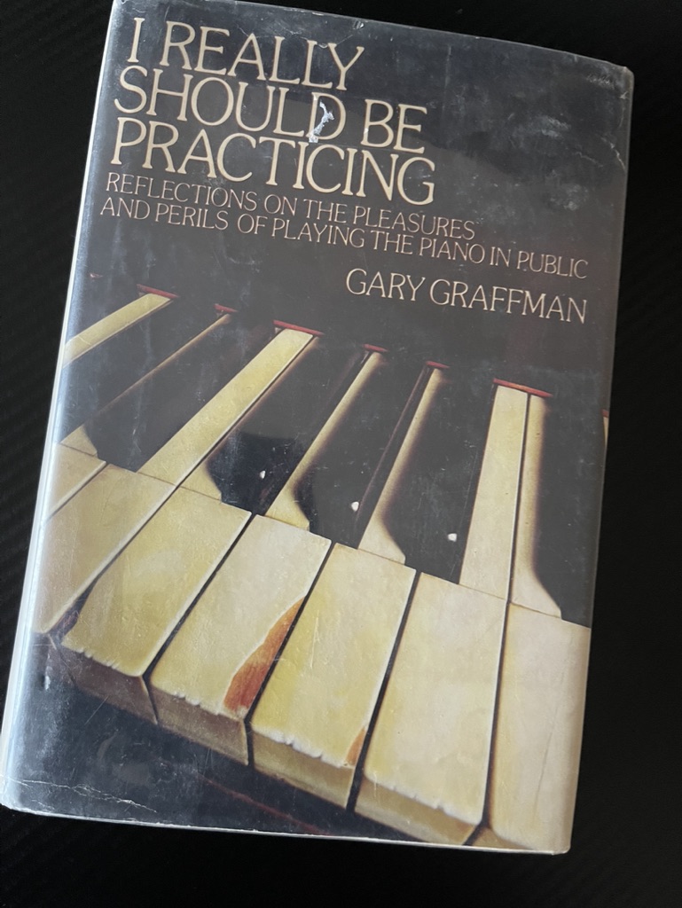
357. bwv232#
kyrie eleison lord, have mercy
christe eleison christ, have mercy
kyrie eleison christ, have mercy
gloria in excelsis deo glory to god in the highest
et in terra pax and on earth, peace
laudamus te we praise you
gratias agimus tibi we give thanks to you
domine deus, rex coelestis lord god, heavenly king
qui tollis peccata mundi you who take away the sins of the world
qui sedes ad dexteram patrix who sits at the right hand of the father
quoniam tu solus sanctus for you alone are the holy one
cum sancto spiritu with the holy spirit
credo in unum deum i believe in one god
patrem omnipotentum the father almight
et in unum dominum and in one lord
et incarnatus est and was incarnate
crucifixus crucified
et resurrexit and rose again
et in spiritum sanctum and in the holy spirit
confiteor in unum baptisma i confess one baptism
et expecto and i await
sanctus dominus deus sabaoth holy lord god of hosts
osanna in excelsis hosanna in the highest
benedictus qui venit blessed is he who comes
osanna in excelsis hosanna in the highest
agnus dei, qui tollis peccata mundi lamb of god, who takes away the sins of the world
dona nobis pacem grant us peace
Show code cell source
import networkx as nx
import matplotlib.pyplot as plt
import numpy as np
import sklearn as skl

#plt.figure(figsize=[2, 2])
G = nx.DiGraph()
G.add_node("Cosmos ",  pos = (0, 5) )
G.add_node("Quake",  pos = (1, 5) )
G.add_node("Flood",  pos = (2, 5) )
G.add_node("Plague",  pos = (3, 5) )
G.add_node("Vexed",  pos = (4, 5) )
G.add_node("Kyrie",  pos = (5, 5) )
G.add_node("Eleison",  pos = (6, 5) )
G.add_node("Christe",  pos = (7, 5) )

G.add_node("Yhwh",  pos = (1.4, 4) )
G.add_node("Father",  pos = (2.8, 4) )
G.add_node("Son",  pos = (4.2, 4) )
G.add_node("Holy",  pos = (5.6, 4) )

G.add_node("Literal",  pos = (2.1, 3) )
G.add_node("Methaph",  pos = (4.9, 3) )

G.add_node("Covenat",  pos = (1.4, 2) )
G.add_node("Lamb",  pos = (2.8, 2) )
G.add_node("Wine",  pos = (4.2, 2) )
G.add_node("Bread",  pos = (5.6, 2) )


G.add_node("Ark",  pos = (0, 1) )
G.add_node("War",  pos = (1, 1) )
G.add_node("Requite",  pos = (2, 1) )
G.add_node("Discord",  pos = (3, 1) )
G.add_node("Forever",  pos = (4, 1) )
G.add_node("God",  pos = (5, 1) )
G.add_node("With",  pos = (6, 1) )
G.add_node("Tobe",  pos = (7, 1) )

G.add_edges_from([ ("Cosmos ", "Yhwh"),  ("Cosmos ", "Father"),  ("Cosmos ", "Son"),  ("Cosmos ", "Holy")])
G.add_edges_from([ ("Quake", "Yhwh"),  ("Quake", "Father"),  ("Quake", "Son"),  ("Quake", "Holy")])
G.add_edges_from([ ("Flood", "Yhwh"),  ("Flood", "Father"),  ("Flood", "Son"),  ("Flood", "Holy")])
G.add_edges_from([ ("Plague", "Yhwh"),  ("Plague", "Father"),  ("Plague", "Son"),  ("Plague", "Holy")])
G.add_edges_from([ ("Vexed", "Yhwh"),  ("Vexed", "Father"),  ("Vexed", "Son"),  ("Vexed", "Holy")])
G.add_edges_from([ ("Kyrie", "Yhwh"),  ("Kyrie", "Father"),  ("Kyrie", "Son"),  ("Kyrie", "Holy")])
G.add_edges_from([ ("Eleison", "Yhwh"),  ("Eleison", "Father"),  ("Eleison", "Son"),  ("Eleison", "Holy")])
G.add_edges_from([ ("Christe", "Yhwh"),  ("Christe", "Father"),  ("Christe", "Son"),  ("Christe", "Holy")])

G.add_edges_from([ ("Yhwh", "Literal"),  ("Yhwh", "Methaph")])
G.add_edges_from([ ("Father", "Literal"),  ("Father", "Methaph")])
G.add_edges_from([ ("Son", "Literal"),  ("Son", "Methaph")])
G.add_edges_from([ ("Holy", "Literal"),  ("Holy", "Methaph")])


G.add_edges_from([ ("Literal", "Covenat"),  ("Literal", "Lamb"),  ("Literal", "Wine"),  ("Literal", "Bread")])
G.add_edges_from([ ("Methaph", "Covenat"),  ("Methaph", "Lamb"),  ("Methaph", "Wine"),  ("Methaph", "Bread")])

G.add_edges_from([ ("Covenat", "Ark"),  ("Covenat", "War"),  ("Covenat", "Requite"),  ("Covenat", "Discord")])
G.add_edges_from([ ("Covenat", "Forever"),  ("Covenat", "God"),  ("Covenat", "With"),  ("Covenat", "Tobe")])
G.add_edges_from([ ("Lamb", "Ark"),  ("Lamb", "War"),  ("Lamb", "Requite"),  ("Lamb", "Discord")])
G.add_edges_from([ ("Lamb", "Forever"),  ("Lamb", "God"),  ("Lamb", "With"),  ("Lamb", "Tobe")])
G.add_edges_from([ ("Wine", "Ark"),  ("Wine", "War"),  ("Wine", "Requite"),  ("Wine", "Discord")])
G.add_edges_from([ ("Wine", "Forever"),  ("Wine", "God"),  ("Wine", "With"),  ("Wine", "Tobe")])
G.add_edges_from([ ("Bread", "Ark"),  ("Bread", "War"),  ("Bread", "Requite"),  ("Bread", "Discord")])
G.add_edges_from([ ("Bread", "Forever"),  ("Bread", "God"),  ("Bread", "With"),  ("Bread", "Tobe")])


#G.add_edges_from([("H11", "H21"), ("H11", "H22"), ("H12", "H21"), ("H12", "H22")])
#G.add_edges_from([("H21", "Y"), ("H22", "Y")])
nx.draw(G,
        nx.get_node_attributes(G, 'pos'),
        with_labels=True,
        font_weight='bold',
        node_size = 3000,
        node_color = "lightblue",
        linewidths = 3)
ax= plt.gca()
ax.collections[0].set_edgecolor("#000000")
ax.set_xlim([-.5, 7.5])
ax.set_ylim([.5, 5.5])
plt.show()
---------------------------------------------------------------------------
ModuleNotFoundError                       Traceback (most recent call last)
Cell In[1], line 1
----> 1 import networkx as nx
      2 import matplotlib.pyplot as plt
      3 import numpy as np

ModuleNotFoundError: No module named 'networkx'
359. mozart#
domino deus is my fave from mass in c
but the kyrie-christe-kyrie might be a close second
or perhaps they tie? granted, the credo brings some memories!!
were i more firm in my credo those painful memories might have been of victory!!!
just realized that i’ve to distinguish
credo: credo in unum deumfromcredo: et incarnatus estoh boy. mozart b winning. bach & ludwig stand no chance if we are to go by
stealing the heart, zero competitionanyways:
otherwise; i wish to discuss with you — much later — the possibility of having a listening session for musical interpretations of Latin mass by Bach, Mozart & Beethoven. I’ve been doing this by myself (pretty lonely) for the last 17 years. But if there are enthusiasts for Latin mass like you, it would open up the chance to share this very rich pedigree from the 17th & 18th century Prussia
360. !chronological#
senses: mozart
mind: bach
flex: beethoven
361. vanguard#
its taken them this long to go live?
find time to investigate why
anyways, they’re here…
362. große messe#
372. unfinished#
mozarts mass
schuberts symphony in b minor
i don’t care what the composers themselves say
these are complete works
absolutely nothing is unfinished
only the view of
genreimpossed this title
große messe is the only mass that draws blood
bachs and ludwigs are masterpieces but
only from a cerebral or flex stance
373. gloria#
mozarts gloria: qui tollis
obviously written while he studied handel
recalls handel’s messiah: overture & more
374. autoencoding#
works of art
representation
same idea but for algorithms
to imitate is to interpret, world meaningfully
375. autoencode#
encode
encyclopedia
western
styles, forms, procedures
-
musical offering
the art of fugue
b minor mass
decode
we know of no occasion for which bach could have written the b-minor mass, nor any patron who might have commissioned it, nor any performance of the complete work before 1750
376. schubert#
how stand i then?
06/02/2023#
377. esot#
plan
go
378. service#
full of vexation come i, with complaint
kyrielauded service provider
gloriaessence of offering
credothe quality of service
sanctusour goal is to have a happy customer!
agnus dei
379. vivaldi#
what does it say of him that his best liturgical work is
gloria in d?do any of his descendants surpass the spirit of praise in
domine fili unigenite?his
domine deus, rex coelestismight as well be by bach, his descendant!can’t fault him for range: the two gloria pieces above straddle a wide range of emotions
i think vivaldi & handel were the last bastilon of light, tight instrumentation
those were the days when instumentation was nothing more than support for voice
380. laudate#
mozart’s vesperae solennes de confessore in c, k.339
psalm 116/117
o praise the lord, all ye nations
praise him, all ye people
from time to time god must feel mercy on humanity
and so he sent an angel: wolfgang ama-
deusmozart. and …now another heavenly voice: barbara hendricks
there is no other explanation for such wonder of sound, the direct key to our soul! – youtuber comment
381. automation#
how autoencoding is basis for all of mankinds progress
encode essence of human services (e.g., bank teller)
code to replicate process (e.g., SAS, etc)
decode service delivery (e.g. atm)
witnessed similar process at ups store today:
place order online
showup to print label
bypass those in line
just dropoff
voila!
382. workflow#
autoencode with vincent
extract very essence
then iterate!!!
383. drugs&aging#
384. atc#
june 5
arrive
june 6
amy talk
june 7
depart
385. feedback#
most detailed feedback
from department of ih
its very rich & a+
Hi Xxx,
This is very detailed and extremely helpful feedback, thanks!
Will also be confirming on Monday whether I’ll be able to have you as TA this summer.
But for next spring, you are already booked if you’re still interested!
Yo
From: Xxx Xxx xxx123@jhmi.edu
Date: Friday, June 2, 2023 at 7:20 AM
To: Yours Truly truly@jhmi.edu
Subject: Feedback on STATA programming_xxxxx
Hi Yo,
I hope this message finds you well. As a student in your recent STATA programming course, I am taking this opportunity to share my feedback. Please understand this is offered constructively, and I truly appreciate your dedication to teaching this course. It has been a valuable learning experience for me.
Also if you still have time, you can send me specific questions and I can answer them again.
Course Introduction for Novices:
The first lecture appeared to be quite advanced, and this proved to be a challenging starting point for those new to STATA. I still remember on the first day of the class, a bunch of “horrible” coding has been shown, and one of my classmates told me that she would quit the course as she cannot understand most of the knowledge of the first lecture. I believe the course could benefit from a simpler code introduction in the first class, to ease new users into the platform and set them up for future success.Code Complexity:
There were times when the complexity of the code made comprehension difficult for some students. As I think the primary goal is to help students understand the logic of commands, it might be beneficial to break down complex coding sequences into simpler steps, or to provide more detailed explanations of complicated code. The complicated codes and example can be introduced if most students understand the logic.Github Organization: The Github repository for the course could potentially be more intuitively organized, which would make it easier for students to locate and utilize course resources (e.g: sometimes it can be difficult to find the corresponding codes just based on the content table).
Syllabus Structure: While the syllabus provided an overview of the course, a more detailed, organized structure would help students prepare better for each session and understand the progression of the course (What will be done in this week? What is the goal of today’s session? Which commands will be taught today? These can be listed on Github)
TA Availability: The class could greatly benefit from additional TA support, particularly during live in-person sessions. This would allow for more immediate responses to student queries and might enhance the overall learning experience.
STATA Logic Session: Incorporating a session dedicated to explaining the logic of STATA could help students grasp the reasoning behind certain programming methods and better understand how to apply them in their own work (e.g: when STATA is more convenient than other statistical language? How to find STATA resources if meet problems? How to manage the database of STATA?)
Practice Questions: The inclusion of ungraded practice problems after each session could be a useful way for students to apply the newly learned knowledge and skills. This could also help reinforce the key takeaways from each lesson.
Overall, your course has been immensely insightful and provided me with an array of new techniques and a deeper understanding of STATA. I believe these suggestions might help to further refine the course for future cohorts.
Thank you for your understanding, and I appreciate your open-mindedness to student feedback. I look forward to continuing to learn from your expertise in future courses.
Best regards,
Xxx Xx
Show code cell source
import networkx as nx
import matplotlib.pyplot as plt
import numpy as np
import sklearn as skl

#plt.figure(figsize=[2, 2])
G = nx.DiGraph()
G.add_node("Cosmos ",  pos = (0, 5) )
G.add_node("Quake",  pos = (1, 5) )
G.add_node("Flood",  pos = (2, 5) )
G.add_node("Plague",  pos = (3, 5) )
G.add_node("Vexed",  pos = (4, 5) )
G.add_node("Kyrie",  pos = (5, 5) )
G.add_node("Eleison",  pos = (6, 5) )
G.add_node("Christe",  pos = (7, 5) )

G.add_node("Yhwh",  pos = (1.4, 4) )
G.add_node("Father",  pos = (2.8, 4) )
G.add_node("Son",  pos = (4.2, 4) )
G.add_node("Holy",  pos = (5.6, 4) )

G.add_node("Literal",  pos = (2.1, 3) )
G.add_node("Methaph",  pos = (4.9, 3) )

G.add_node("Covenat",  pos = (1.4, 2) )
G.add_node("Lamb",  pos = (2.8, 2) )
G.add_node("Wine",  pos = (4.2, 2) )
G.add_node("Bread",  pos = (5.6, 2) )


G.add_node("Ark",  pos = (0, 1) )
G.add_node("War",  pos = (1, 1) )
G.add_node("Requite",  pos = (2, 1) )
G.add_node("Discord",  pos = (3, 1) )
G.add_node("Forever",  pos = (4, 1) )
G.add_node("God",  pos = (5, 1) )
G.add_node("With",  pos = (6, 1) )
G.add_node("Tobe",  pos = (7, 1) )

G.add_edges_from([ ("Cosmos ", "Yhwh"),  ("Cosmos ", "Father"),  ("Cosmos ", "Son"),  ("Cosmos ", "Holy")])
G.add_edges_from([ ("Quake", "Yhwh"),  ("Quake", "Father"),  ("Quake", "Son"),  ("Quake", "Holy")])
G.add_edges_from([ ("Flood", "Yhwh"),  ("Flood", "Father"),  ("Flood", "Son"),  ("Flood", "Holy")])
G.add_edges_from([ ("Plague", "Yhwh"),  ("Plague", "Father"),  ("Plague", "Son"),  ("Plague", "Holy")])
G.add_edges_from([ ("Vexed", "Yhwh"),  ("Vexed", "Father"),  ("Vexed", "Son"),  ("Vexed", "Holy")])
G.add_edges_from([ ("Kyrie", "Yhwh"),  ("Kyrie", "Father"),  ("Kyrie", "Son"),  ("Kyrie", "Holy")])
G.add_edges_from([ ("Eleison", "Yhwh"),  ("Eleison", "Father"),  ("Eleison", "Son"),  ("Eleison", "Holy")])
G.add_edges_from([ ("Christe", "Yhwh"),  ("Christe", "Father"),  ("Christe", "Son"),  ("Christe", "Holy")])

G.add_edges_from([ ("Yhwh", "Literal"),  ("Yhwh", "Methaph")])
G.add_edges_from([ ("Father", "Literal"),  ("Father", "Methaph")])
G.add_edges_from([ ("Son", "Literal"),  ("Son", "Methaph")])
G.add_edges_from([ ("Holy", "Literal"),  ("Holy", "Methaph")])


G.add_edges_from([ ("Literal", "Covenat"),  ("Literal", "Lamb"),  ("Literal", "Wine"),  ("Literal", "Bread")])
G.add_edges_from([ ("Methaph", "Covenat"),  ("Methaph", "Lamb"),  ("Methaph", "Wine"),  ("Methaph", "Bread")])

G.add_edges_from([ ("Covenat", "Ark"),  ("Covenat", "War"),  ("Covenat", "Requite"),  ("Covenat", "Discord")])
G.add_edges_from([ ("Covenat", "Forever"),  ("Covenat", "God"),  ("Covenat", "With"),  ("Covenat", "Tobe")])
G.add_edges_from([ ("Lamb", "Ark"),  ("Lamb", "War"),  ("Lamb", "Requite"),  ("Lamb", "Discord")])
G.add_edges_from([ ("Lamb", "Forever"),  ("Lamb", "God"),  ("Lamb", "With"),  ("Lamb", "Tobe")])
G.add_edges_from([ ("Wine", "Ark"),  ("Wine", "War"),  ("Wine", "Requite"),  ("Wine", "Discord")])
G.add_edges_from([ ("Wine", "Forever"),  ("Wine", "God"),  ("Wine", "With"),  ("Wine", "Tobe")])
G.add_edges_from([ ("Bread", "Ark"),  ("Bread", "War"),  ("Bread", "Requite"),  ("Bread", "Discord")])
G.add_edges_from([ ("Bread", "Forever"),  ("Bread", "God"),  ("Bread", "With"),  ("Bread", "Tobe")])


#G.add_edges_from([("H11", "H21"), ("H11", "H22"), ("H12", "H21"), ("H12", "H22")])
#G.add_edges_from([("H21", "Y"), ("H22", "Y")])
nx.draw(G,
        nx.get_node_attributes(G, 'pos'),
        with_labels=True,
        font_weight='bold',
        node_size = 3000,
        node_color = "lightblue",
        linewidths = 3)
ax= plt.gca()
ax.collections[0].set_edgecolor("#000000")
ax.set_xlim([-.5, 7.5])
ax.set_ylim([.5, 5.5])
plt.show()
plague, vexation
service, evaluation
codify, basics
decode, telemedicine
happyness, pondereplay
387. badgyalriri#
now i’ve just watched pon de replay video and was struck at 2:30/3:37
does beyoncé have any formation-style choreography like this before 2005?
she certainly has
a lotof it later; if none before 2005, then she totally stole the idea from badgalririof course we are not suggesting that originality is a thing; we’re merely tracking the creative process
388. teach!#
man/data
artist/encode
work/code
critic/decode
spectator/knowledge
path
maze
labyrinth
darkness
forward
light
guide
shepherd
annuŋŋamya
decisions
policy
guidelines
rx
389. beyoncé#
she codifies
a lotfeminism
black power
empowerment
will-to-power
kulture
slay ⚔
390. scalability#
code -> decode
that is what is scalable
and is the very essence of progress
391. growth#
autoencode
scale
grow
dominate
legacy
392. funny#
might aphrodite
essence of great art:
we suffer and perish so that poets may not lack material
393. stata#
vs @code
code editing
redefined?
even4stata?
investigate!
394. encode#
what do the following encode?
clearly they
dogiven their growth marketsand their presence in my mature life beyond 35yo
weinestaphaner hefe weissbier
westmalle dubel, tripel
duvel
orval
bozal
glenfiddich 15yo solera
lagavulin 16yo
395. kyrie#
k. 626
a whole ‘nother mozart!
the gods can’t let such a fella into old age
396. instrumentation#
how light the instrumention of the requem is!
mozart only presents the essence
its all encoded here
06/03/2023#
397. air#
no coincidence
year of
23film release
398. conventions#
These have been imposed on me by an apparent restraint. When I attempted systematized workdir (340y23s) and repo (600y23s) names it just didn’t work – process was arrested at git push or ghp-import. But simple non-numeric names (workdir: summer & repo: livre) worked seamlessly. And so, just like Apple names its MacOSX versions after some aspect of Californias natural resources (mountains, parks, wildlife), I’ll name my workdir and repo versions each year after some theme and variation (workdir: season & repo: book).
usernames
jhustata
jhutrc
jhusurgery
workdir
seasons
english
spanish
italian
french
german
zulu
yoruba
lusoga
repo
book
english
spanish
italian
french
german
zulu
yoruba
lusoga
399. wayne#
wed june 7 is last day of atc
fly out of lax on thursday
or perhaps out of john wayne?
fa parents visiting currently
but apparently they’ll love me
then tue june 6 is for amy: 18:00-18:10
and mon june 5 is for tijuana
so last sunday flight out west?
400. paulo#
must leave nj june 8th
so may leave ca june 7th
but really tijuana is june 5th
and so ok to leave june 6th
lets spend nites of june 4th, 5th
departure on 6th for both of us to md/n
wild card: stay 6th + john wayne departure
401. trip#
delta #F6JLMG
indigo #9140649956387
402. sq-foot#
indigo
350
waverly
700
other
1500
403. woody allen#
cacophony
ensemble cast of a-listers
one might codify the essence of human life
he’s still a type-i artist:
federico fellini’s catholicism
ingmar bergman’s nordic agnosticism
judaism: ancient, modern, new yorker
greek mythology, philosophy, talmud
uses these moulds for dramatis personnae
as a template for neurotic nyc types
of course his greatest success is navel-gazing
because he’s lots of material from his own existential pangs
404. ghp-import#
when stuck at
git pushofghp-importdiagnose cause: often corrupted image
so get rid of it and empty cloned repo
you’d
cp -r jupyter-book/* repoanywaysthis may spare you untold misery
405. love#
who can i run to?
xscape ask the question!
bewildering array of emotions
and potential guarantor
of peace, calm
what else is this but dimensionality reduction?
from \(\infty\) -> X=1?
dull!
06/04/2023#
406. annuŋŋamya#
original version
by ayf’s
jessica mirembe
407. neat#
we know
fifth harmony
not too shabby
but wrong reason
to get entire album!
408. r.kelly#
if you dream
clearly inspired
by storm is over by the r in r&b
probably written by tank and j valentine
tank
tyrese
toni braxton
jordin sparks
omario
faith evans
jojo
charlie wilson
tamar braxton
steve russell
rather beautiful song
sound track like its inspiration
06/07/2023#
409. feedback#
be sure to analyse it
i didn’t know how to access it
now that i see the 2021/2022 feedback
clear that i perpetuated the issues and added more
this has been all too little, too late for the graduates
however, i’ll be responsive even as early as this summer
gentle learning curve
organized content
relevant to homework
early feedback
competent teaching assistants
avoid humor since its really mockery
difference between tragedy & comedy 🎭?
we don’t empathize with the victim in comedy
yet we do with the one in tragedy
a student is the victim
students recommend that i get more professional
one resource for that
410. summary#
“Like all people who try to exhaust a subject, he exhausted his listeners.”
― Oscar Wilde, The Picture of Dorian Gray
411. boring#
in-class tasks
write program
that does …
assistants present
use python figure
412. engaging#
introduce essence of idea in 10min
practice that in-class
then link that to homework
perhaps reverse engineer process
start with homework & think: what skill
class is about providing technical skill to do hw
413. man#
data - man delights, not me
encode - invariable progression to death
code - solomon, hamlet, macbeth, elementary particles
decode - detraction will not suffer it (delights)
represent - and so i end my catechism
414. ysidro#
uber to san ysidro
walk across boarder
will fillout a brief form
option: mercado m. hidalgo
then uber to rosarito
maybe do revolucion at nite
spend additional nite?
caesars restaurant next day
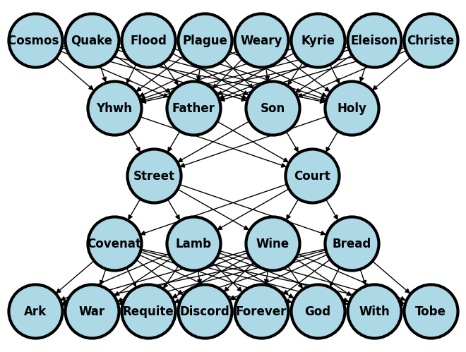
415. catechism#
Show code cell source
import networkx as nx
import matplotlib.pyplot as plt
import numpy as np
import sklearn as skl

#plt.figure(figsize=[2, 2])
G = nx.DiGraph()
G.add_node("Cosmos ",  pos = (0, 5) )
G.add_node("Quake",  pos = (1, 5) )
G.add_node("Flood",  pos = (2, 5) )
G.add_node("Plague",  pos = (3, 5) )
G.add_node("Vexed",  pos = (4, 5) )
G.add_node("Kyrie",  pos = (5, 5) )
G.add_node("Eleison",  pos = (6, 5) )
G.add_node("Christe",  pos = (7, 5) )

G.add_node("Yhwh",  pos = (1.4, 4) )
G.add_node("Father",  pos = (2.8, 4) )
G.add_node("Son",  pos = (4.2, 4) )
G.add_node("Holy",  pos = (5.6, 4) )

G.add_node("Q",  pos = (2.1, 3) )
G.add_node("A",  pos = (4.9, 3) )

G.add_node("Covenat",  pos = (1.4, 2) )
G.add_node("Lamb",  pos = (2.8, 2) )
G.add_node("Wine",  pos = (4.2, 2) )
G.add_node("Bread",  pos = (5.6, 2) )


G.add_node("Ark",  pos = (0, 1) )
G.add_node("War",  pos = (1, 1) )
G.add_node("Requite",  pos = (2, 1) )
G.add_node("Discord",  pos = (3, 1) )
G.add_node("Forever",  pos = (4, 1) )
G.add_node("God",  pos = (5, 1) )
G.add_node("With",  pos = (6, 1) )
G.add_node("Tobe",  pos = (7, 1) )

G.add_edges_from([ ("Cosmos ", "Yhwh"),  ("Cosmos ", "Father"),  ("Cosmos ", "Son"),  ("Cosmos ", "Holy")])
G.add_edges_from([ ("Quake", "Yhwh"),  ("Quake", "Father"),  ("Quake", "Son"),  ("Quake", "Holy")])
G.add_edges_from([ ("Flood", "Yhwh"),  ("Flood", "Father"),  ("Flood", "Son"),  ("Flood", "Holy")])
G.add_edges_from([ ("Plague", "Yhwh"),  ("Plague", "Father"),  ("Plague", "Son"),  ("Plague", "Holy")])
G.add_edges_from([ ("Vexed", "Yhwh"),  ("Vexed", "Father"),  ("Vexed", "Son"),  ("Vexed", "Holy")])
G.add_edges_from([ ("Kyrie", "Yhwh"),  ("Kyrie", "Father"),  ("Kyrie", "Son"),  ("Kyrie", "Holy")])
G.add_edges_from([ ("Eleison", "Yhwh"),  ("Eleison", "Father"),  ("Eleison", "Son"),  ("Eleison", "Holy")])
G.add_edges_from([ ("Christe", "Yhwh"),  ("Christe", "Father"),  ("Christe", "Son"),  ("Christe", "Holy")])

G.add_edges_from([ ("Yhwh", "Q"),  ("Yhwh", "A")])
G.add_edges_from([ ("Father", "Q"),  ("Father", "A")])
G.add_edges_from([ ("Son", "Q"),  ("Son", "A")])
G.add_edges_from([ ("Holy", "Q"),  ("Holy", "A")])


G.add_edges_from([ ("Q", "Covenat"),  ("Q", "Lamb"),  ("Q", "Wine"),  ("Q", "Bread")])
G.add_edges_from([ ("A", "Covenat"),  ("A", "Lamb"),  ("A", "Wine"),  ("A", "Bread")])

G.add_edges_from([ ("Covenat", "Ark"),  ("Covenat", "War"),  ("Covenat", "Requite"),  ("Covenat", "Discord")])
G.add_edges_from([ ("Covenat", "Forever"),  ("Covenat", "God"),  ("Covenat", "With"),  ("Covenat", "Tobe")])
G.add_edges_from([ ("Lamb", "Ark"),  ("Lamb", "War"),  ("Lamb", "Requite"),  ("Lamb", "Discord")])
G.add_edges_from([ ("Lamb", "Forever"),  ("Lamb", "God"),  ("Lamb", "With"),  ("Lamb", "Tobe")])
G.add_edges_from([ ("Wine", "Ark"),  ("Wine", "War"),  ("Wine", "Requite"),  ("Wine", "Discord")])
G.add_edges_from([ ("Wine", "Forever"),  ("Wine", "God"),  ("Wine", "With"),  ("Wine", "Tobe")])
G.add_edges_from([ ("Bread", "Ark"),  ("Bread", "War"),  ("Bread", "Requite"),  ("Bread", "Discord")])
G.add_edges_from([ ("Bread", "Forever"),  ("Bread", "God"),  ("Bread", "With"),  ("Bread", "Tobe")])


#G.add_edges_from([("H11", "H21"), ("H11", "H22"), ("H12", "H21"), ("H12", "H22")])
#G.add_edges_from([("H21", "Y"), ("H22", "Y")])
nx.draw(G,
        nx.get_node_attributes(G, 'pos'),
        with_labels=True,
        font_weight='bold',
        node_size = 3000,
        node_color = "lightblue",
        linewidths = 3)
ax= plt.gca()
ax.collections[0].set_edgecolor("#000000")
ax.set_xlim([-.5, 7.5])
ax.set_ylim([.5, 5.5])
plt.show()
416. autoencoder#
nietzsche — he misunderstood the effects of “autoencoding” when he said this: sebastian bach.—in so far as we do not hear bach’s music as perfect and experienced connoisseurs of counterpoint and all the varieties of the fugal style (and accordingly must dispense with real artistic enjoyment), we shall feel in listening to his music—in goethe’s magnificent phrase—as if “we were present at god’s creation of the world.” in other words, we feel here that something great is in the making but not yet made—our mighty modern music, which by conquering nationalities, the church, and counterpoint has conquered the world. in bach there is still too much crude christianity, crude germanism, crude scholasticism. he stands on the threshold of modern european music, but turns from thence to look at the middle ages.
bach is code, essence, from whence the well-tempered clavier, all keys, and all music may be derived. even he occasionally wrote sweet decoded music, as we see in his arias
that said, goethe & nietzsche are generally right in their assessment
417. jesus#
messianic complex
when you figure out
essence of man’s predicament
and offer yourself as palliative
call it altruism, it’s sweet
variants?
parent
spouse
teacher
employer
provider (service)
firm
government
culture
religion
cause
king caesar
how do artists fit in? they teach us
precedence
convention
restraint
teach us dimensionality dedication
lead us towards
?X=1
and that’s how music is the greatest of man’s inventions: how man reduces all cosmic noise to 12 relative frequencies! or to one diatonic key (wherein a chromatic scale of 24 frequencies fit), on a well-tempered clavier!!!
note: one can derive 23 of the 24 relative frequencies given only one of them (typically the tonic). so it’s really one degree of freedom: X=1 (without the ?)
418. crave#
dimensionality reduction
because we are low energy
frailty symptom of human race
419. antithesis#
dionysus visited his uncle hades
found achilles regretting his heroism
looks like earthly achievements are not
currency in hades (no time-varying weight neither)
420. tribe#
strength of a tribe
deduced from number of gods
in their mythology
by extension, the decline
of a tribe may be deduced from
a trend towards fewer explanatory factors
here monotheisim represents the very weakest
most decadent state; by extension, the most intelligent, resentful
using this formula one may productively launch into genealogy of morality
421. s&p#
sobrero
poncho
422. autoencode#
life
bible
mass
magesterium
catholicism
why romans enduringly more successful than greco-judaism
going purely by numbers, territory, and calendar
dimensionality reduction
something every [weak] man craves
thus power to collect indulgences
conquered hearts are easier to manage
otherwise stronger armies necessary, which romans also had
but found this a more efficient system
423. sandiego#
market & 9th
is my kinda joint
so many reasons
424. stream#
of consciousness
sensory impressions
incomplete ideas
unusual syntax
rough grammar
my style for 340.600
according to one student
this was no complement
425. impressions#
sensory
data
input
system
feedback
negative
cripples
if not regulated
but ultimately corrects
output users find unhelpful
how to do it without depressing system!
be more sympathetic to the prudent stance:
hideth
426. hotel#
350 sq foot with city views
750 sq foot < my waverly joint
900 sq foot apt at waverly?
427. piers#
an unlikely topic
but great discussion
highlighting summary statistics
data
encoded
coded (\(\mu, \sigma\))
decoded
inference
anecdotes
misleading
tails of distribution
nonetheless critical info
very skewed distribution say
customer tastes have little variation
perhaps outcome of the capitalistic process
of mass producing, advertizing, scale, autoencoding
428. desensitization#
childhood exposures
result in robust immunity
thus treatment of offensive messengers?
even more free, at times offensive speeach!
my starting poing when it comes to the consideration of any issue relating to free speech is my passionate belief that the second most precious thing in life is hte right to express yourself freely.
the most precious thing in life, i think, is food in your mouth and teh third most precious is a roof oer your head, but a fixture for me in the number 2 slot is free expression, just below the need to sustain life itself. that is because i have enjoyed free expression in this country all my professional life
\(\vdots\)
you might call the new intolerance, a new but intense desire to gag uncomfortable voices of dissent
replacement of one kind of intolerance with another \(\cdots\)
underlying prejudices, injustices or resentments are not addressed by arresting people. they are addressed by the issues being being aired, argued and dealth with preferably outside the legal process. for me, the best way to increase society’s resistance to insulting or offensive speech is to allow a lot more of it.
as with childhood diseases, you can better resist those germs to which you have been exposed. we need to build our immunity to taking offence, so that we can deal with the issues that perfectly justified criticism can raise. our priority should be to deal with message, not the messenger.
president obama said in an address to the united nations, ‘laudable efforts to restrict speech can become a tool to silence critics (goal of an oppossing credo, fyi) or oppress minorities (which is contextual). the strongest weapon against hateful speech is not oppression, it is more speech.]
429. teaching#
no different than art
create boundaries
limit the material
don’t be exhaustive:
dr.more restraint than predecessors!
have constant feedback from students
don’t wait for course eval
thats too little, too late
06/08/2023#
430. monica#
new york directly south of ottawa
started off with banter
about where she is from & school
feedback on the event at which i attended
wants to give me broader strokes on indexes
two-day event: the american dream experience
in terms of added value to my life
covering the last 30 years of my life
$15m in ug gov bonds
$250k in ml playground: controlled experiment
$XX? no clue
she’s set me on calendar for june 2024
431. analysts#
woody allen’s treatment of pyscholanalysts is similar to his treatment of god: willing but not able
or perhaps that god is uninterested, maybe because also not able
but he never questions the existence of analyts: he visited one weekly for 15 years
432. tasks#
program define
syntax varlist
exit 340
display
quietly
433. veritas#
tom hanks at harvard: 19:34/22:16
one of 3-types of americans
embrace liberty & freedom for all
whineth(muscle, efferent blockage)those who won’t
tameth(strong, unconscious type with little cognitive development)and those who are indifferent
hideth(sensory, afferent blockade)
codified the essence of the life tom & i have lived: a sort of external validation
434. liberabit#
and there’s three types of students:
those who leverage innovation, warts & all
tamethcan enumerate instances wherein they were maligned
whinethprudent who are trying to meet the requirements of their program
hideth
cater to all three and give them maximum value
my original preference for type-1 was an unconscious bias
435. generalize#
input
hidethkeyboard
mouse
voice
touch
processor
whinethmainframe
desktop
laptop
cellphone
etc
output
tamethmusic
pictures
documents
etc
436. versus#
437. apple#
dream it
chase it
code it
438. suigeneris#
hardware
software
services
something only apple could do
439. mac#
mac studio
plus apple monitor
incredible performance
connectivity with m2 max
developing new versions of apps
before they go live
hosting after they go live
exploring those options from ds4ph
taking demanding workflows to the next levelm-dimensional simulation is faster than ever
and may use 7 input feeds & encode them
decode and simulate in record time
440. stata#
1
tamethworkflow2
whinethprogram define3
hidethadvanced syntax
these could represent three classes 340.600, 340.700, 340.800
one class sticks to stata programming & the program define command, syntax varlist, etc.
another class introduces advanced syntax that contibutes to quality of the programs from the basic class
finally there is a class that emphasizes workflow, github, collaboration, self-publication
while i may not have time to write up three syllabuses, i could use markdown header-levels to denote these
06/09/2023#
441. apple#
lots of ai/ml lingua
only notice since ds4ph
what luck, my gtpci phd!
442. not-for-profit#
efficiency not prized
increased expenditure is the thing
this is show-cased to win yet more grants
443. psychology#
stable
erratic
pattern
444. program#
stata programming at jhu
444.1 stata i (basic stata 340.600)#
program define myfirst
    di "my first program"
end

myfirst
. program define myfirst
1.     di "my first program"
2. end

.
. myfirst
my first program

.
end of do-file

.
444.2 stata ii (intermediate stata 340.700)#
program define mysecond
    foreach v of varlist init_age peak_pra prev female receiv {
		qui sum `v', d
		di r(mean) "(" r(sd)  ")" ";" r(p50) "(" r(p25) "-" r(p75) ")"
	}
end

clear
import delimited https://raw.githubusercontent.com/jhustata/book/main/hw1.txt
mysecond
. program define mysecond
1.     foreach v of varlist init_age peak_pra prev female receiv {
2.                 qui sum `v', d
3.                 di r(mean) "(" r(sd)  ")" ";" r(p50) "(" r(p25) "-" r(p75)	")"
4.         }
5. end

.
.
.
. clear

. import delimited https://raw.githubusercontent.com/jhustata/book/main/hw1.txt
(encoding automatically selected: ISO-8859-1)
(8 vars, 1,525 obs)

. mysecond
50.575743(14.524256);52.950001(40.549999-61.85)
20.011155(33.867173);0(0-28.5)
.11737705(.32197462);0(0-0)
.38688525(.48719678);0(0-1)
.35147541(.4775877);0(0-1)

.
end of do-file

.
444.3 stata iii (advanced stata 340.800)#
qui do https://raw.githubusercontent.com/muzaale/book/main/mysecond.ado
import delimited https://raw.githubusercontent.com/jhustata/book/main/hw1.txt
mysecond
. clear

. import delimited https://raw.githubusercontent.com/jhustata/book/main/hw1.txt
(encoding automatically selected: ISO-8859-1)
(8 vars, 1,525 obs)

. mysecond
50.575743(14.524256);52.950001(40.549999-61.85)
20.011155(33.867173);0(0-28.5)
.11737705(.32197462);0(0-0)
.38688525(.48719678);0(0-1)
.35147541(.4775877);0(0-1)

.
end of do-file

.
445. in-person#
selective feedback from the in-person students (offered me realtime, but biased feedback)
most complaints from the students who relied on recorded lectures (offered feedback that was too little, too late)
but at the end of the day there are three-types of students & i must recognize that (maybe go beyond .01 and consider…)
446. will-to-power#
is the code of life; everything else represents decoded “consequences” of this fact
there are:
worthy adversaries (type-i)
tameth;others that whine about unfairness of competition (type-ii)
whineth; and,many who are indifferent (type-iii)
hideth
adults will have to choose their lot at some point
447. in-other-words#
unworthy adversaries are the lot of many modern types who consider worthy types as evil incarnate (type-i)
they’re passionate about some cause & have the
will-to-whineon behalf of the school of resentment (type-ii)make no mistake: they consider indifferent types as a subtle but perhaps more problematic enemy of the two (type-iii)
448. autoencode-cipher#
human condition
shakespeare
nietzsche
philosophy
why so hard!
449. requite#
type-i people can requite (
tameth, worthy adversaries, strong)type-ii people resort to whining (
whineth, weary, weak, meek, damsels-in-distress)type-iii people are indifferent (
hideth, prudent, epicurus, god, psychoanalysts, hedonists, etc.)
450. hanks#
those who have grown weary become indifferent and resort to fantasy, superheroes, video games, and other mostly hedonistic distractions such as alcohol, women, and sports
451. weary#
matt 11:28
come unto me, all ye that labor and are heavy laden, and i will give you rest
psalm 23
the lord is my shepherd; i shall not want.

he maketh me to lie down in green pastures: he leadeth me beside the still waters.

he restoreth my soul: he leadeth me in the paths of righteousness for his name's sake.

yea, though I walk through the valley of the shadow of death, i will fear no evil: for thou art with me; thy rod and thy staff they comfort me.

thou preparest a table before me in the presence of mine enemies: thou anointest my head with oil; my cup runneth over.

surely goodness and mercy shall follow me all the days of my life: and I will dwell in the house of the Lord for ever.
tom hanks closed with these words:
may goodness and mercy follow you all the days, all the days, of your lives. godspeed!
Show code cell source
import networkx as nx
import matplotlib.pyplot as plt
import numpy as np
import sklearn as skl

#plt.figure(figsize=[2, 2])
G = nx.DiGraph()
G.add_node("Cosmos ",  pos = (0, 5) )
G.add_node("Quake",  pos = (1, 5) )
G.add_node("Flood",  pos = (2, 5) )
G.add_node("Plague",  pos = (3, 5) )
G.add_node("Weary",  pos = (4, 5) )
G.add_node("Kyrie",  pos = (5, 5) )
G.add_node("Eleison",  pos = (6, 5) )
G.add_node("Christe",  pos = (7, 5) )

G.add_node("Yhwh",  pos = (1.4, 4) )
G.add_node("Father",  pos = (2.8, 4) )
G.add_node("Son",  pos = (4.2, 4) )
G.add_node("Holy",  pos = (5.6, 4) )

G.add_node("Q",  pos = (2.1, 3) )
G.add_node("A",  pos = (4.9, 3) )

G.add_node("Covenat",  pos = (1.4, 2) )
G.add_node("Lamb",  pos = (2.8, 2) )
G.add_node("Wine",  pos = (4.2, 2) )
G.add_node("Bread",  pos = (5.6, 2) )


G.add_node("Ark",  pos = (0, 1) )
G.add_node("War",  pos = (1, 1) )
G.add_node("Requite",  pos = (2, 1) )
G.add_node("Discord",  pos = (3, 1) )
G.add_node("Forever",  pos = (4, 1) )
G.add_node("God",  pos = (5, 1) )
G.add_node("With",  pos = (6, 1) )
G.add_node("Tobe",  pos = (7, 1) )

G.add_edges_from([ ("Cosmos ", "Yhwh"),  ("Cosmos ", "Father"),  ("Cosmos ", "Son"),  ("Cosmos ", "Holy")])
G.add_edges_from([ ("Quake", "Yhwh"),  ("Quake", "Father"),  ("Quake", "Son"),  ("Quake", "Holy")])
G.add_edges_from([ ("Flood", "Yhwh"),  ("Flood", "Father"),  ("Flood", "Son"),  ("Flood", "Holy")])
G.add_edges_from([ ("Plague", "Yhwh"),  ("Plague", "Father"),  ("Plague", "Son"),  ("Plague", "Holy")])
G.add_edges_from([ ("Weary", "Yhwh"),  ("Weary", "Father"),  ("Weary", "Son"),  ("Weary", "Holy")])
G.add_edges_from([ ("Kyrie", "Yhwh"),  ("Kyrie", "Father"),  ("Kyrie", "Son"),  ("Kyrie", "Holy")])
G.add_edges_from([ ("Eleison", "Yhwh"),  ("Eleison", "Father"),  ("Eleison", "Son"),  ("Eleison", "Holy")])
G.add_edges_from([ ("Christe", "Yhwh"),  ("Christe", "Father"),  ("Christe", "Son"),  ("Christe", "Holy")])

G.add_edges_from([ ("Yhwh", "Q"),  ("Yhwh", "A")])
G.add_edges_from([ ("Father", "Q"),  ("Father", "A")])
G.add_edges_from([ ("Son", "Q"),  ("Son", "A")])
G.add_edges_from([ ("Holy", "Q"),  ("Holy", "A")])


G.add_edges_from([ ("Q", "Covenat"),  ("Q", "Lamb"),  ("Q", "Wine"),  ("Q", "Bread")])
G.add_edges_from([ ("A", "Covenat"),  ("A", "Lamb"),  ("A", "Wine"),  ("A", "Bread")])

G.add_edges_from([ ("Covenat", "Ark"),  ("Covenat", "War"),  ("Covenat", "Requite"),  ("Covenat", "Discord")])
G.add_edges_from([ ("Covenat", "Forever"),  ("Covenat", "God"),  ("Covenat", "With"),  ("Covenat", "Tobe")])
G.add_edges_from([ ("Lamb", "Ark"),  ("Lamb", "War"),  ("Lamb", "Requite"),  ("Lamb", "Discord")])
G.add_edges_from([ ("Lamb", "Forever"),  ("Lamb", "God"),  ("Lamb", "With"),  ("Lamb", "Tobe")])
G.add_edges_from([ ("Wine", "Ark"),  ("Wine", "War"),  ("Wine", "Requite"),  ("Wine", "Discord")])
G.add_edges_from([ ("Wine", "Forever"),  ("Wine", "God"),  ("Wine", "With"),  ("Wine", "Tobe")])
G.add_edges_from([ ("Bread", "Ark"),  ("Bread", "War"),  ("Bread", "Requite"),  ("Bread", "Discord")])
G.add_edges_from([ ("Bread", "Forever"),  ("Bread", "God"),  ("Bread", "With"),  ("Bread", "Tobe")])


#G.add_edges_from([("H11", "H21"), ("H11", "H22"), ("H12", "H21"), ("H12", "H22")])
#G.add_edges_from([("H21", "Y"), ("H22", "Y")])
nx.draw(G,
        nx.get_node_attributes(G, 'pos'),
        with_labels=True,
        font_weight='bold',
        node_size = 3000,
        node_color = "lightblue",
        linewidths = 3)
ax= plt.gca()
ax.collections[0].set_edgecolor("#000000")
ax.set_xlim([-.5, 7.5])
ax.set_ylim([.5, 5.5])
plt.show()
452. cathecism#
what does it take to produce a table, figure, or abstract like
thisone?output of choice (stata monitor, logfile, excel, word, figure, markdown, html, online)
text (abstract, manuscript, website, catalog)
macros (summaries, estimates, formats, names, embedding)
command to produce output (summary, count, regress)
so, today we are going to focus on
thisaspect!stata monitor
logfile
excel
wordcp
figure
markdown
html
online
later we’ll develop this idea till \(\cdots\)
peer-review ready
beta-testing
etc
453. buzzwords#
thanks to the neuroengine in apple silicon, we now …
api
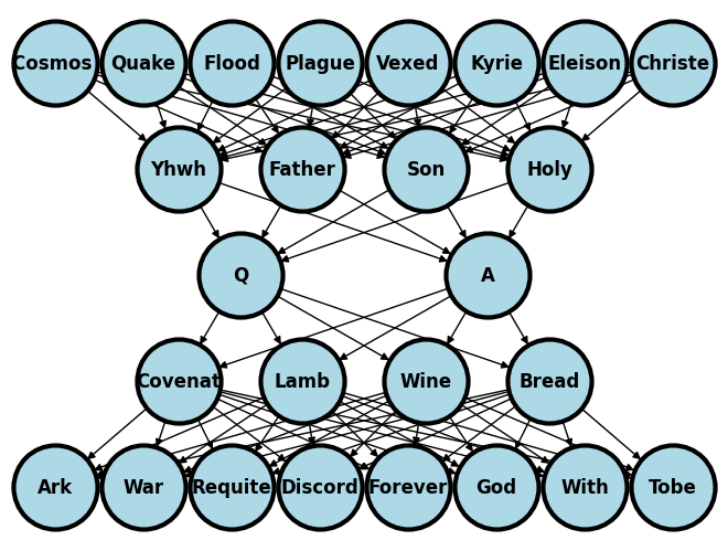
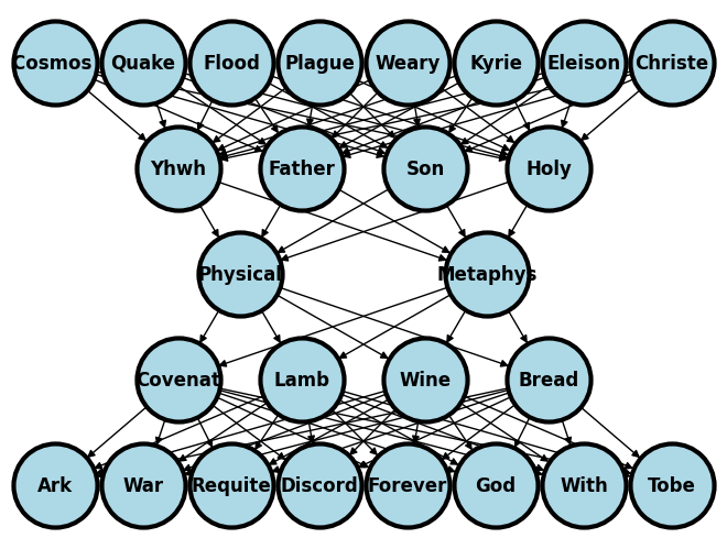
454. visionpro#
augmented reality
digital world
physical space
computer
+ 3d interface: visionpro
+ 2d interface: mac, iphoneoutput
look through it (a first in our products)
input
eyes
voice
hands
use your apps
immersively
on infinite canvas
no longer limited by display
make apps any size you want
revolutions/input
mac -> personal computing/mouse
iphones -> mobile computing/touch-multi
visionpro -> spatial computing/eyes, hands, voice
Show code cell source
import networkx as nx
import matplotlib.pyplot as plt
import numpy as np
import sklearn as skl

#plt.figure(figsize=[2, 2])
G = nx.DiGraph()
G.add_node("Cosmos ",  pos = (0, 5) )
G.add_node("Quake",  pos = (1, 5) )
G.add_node("Flood",  pos = (2, 5) )
G.add_node("Plague",  pos = (3, 5) )
G.add_node("Weary",  pos = (4, 5) )
G.add_node("Kyrie",  pos = (5, 5) )
G.add_node("Eleison",  pos = (6, 5) )
G.add_node("Christe",  pos = (7, 5) )

G.add_node("Yhwh",  pos = (1.4, 4) )
G.add_node("Father",  pos = (2.8, 4) )
G.add_node("Son",  pos = (4.2, 4) )
G.add_node("Holy",  pos = (5.6, 4) )

G.add_node("Real",  pos = (2.1, 3) )
G.add_node("Virtual",  pos = (4.9, 3) )

G.add_node("Covenat",  pos = (1.4, 2) )
G.add_node("Lamb",  pos = (2.8, 2) )
G.add_node("Wine",  pos = (4.2, 2) )
G.add_node("Bread",  pos = (5.6, 2) )


G.add_node("Ark",  pos = (0, 1) )
G.add_node("War",  pos = (1, 1) )
G.add_node("Requite",  pos = (2, 1) )
G.add_node("Discord",  pos = (3, 1) )
G.add_node("Forever",  pos = (4, 1) )
G.add_node("God",  pos = (5, 1) )
G.add_node("With",  pos = (6, 1) )
G.add_node("Tobe",  pos = (7, 1) )

G.add_edges_from([ ("Cosmos ", "Yhwh"),  ("Cosmos ", "Father"),  ("Cosmos ", "Son"),  ("Cosmos ", "Holy")])
G.add_edges_from([ ("Quake", "Yhwh"),  ("Quake", "Father"),  ("Quake", "Son"),  ("Quake", "Holy")])
G.add_edges_from([ ("Flood", "Yhwh"),  ("Flood", "Father"),  ("Flood", "Son"),  ("Flood", "Holy")])
G.add_edges_from([ ("Plague", "Yhwh"),  ("Plague", "Father"),  ("Plague", "Son"),  ("Plague", "Holy")])
G.add_edges_from([ ("Weary", "Yhwh"),  ("Weary", "Father"),  ("Weary", "Son"),  ("Weary", "Holy")])
G.add_edges_from([ ("Kyrie", "Yhwh"),  ("Kyrie", "Father"),  ("Kyrie", "Son"),  ("Kyrie", "Holy")])
G.add_edges_from([ ("Eleison", "Yhwh"),  ("Eleison", "Father"),  ("Eleison", "Son"),  ("Eleison", "Holy")])
G.add_edges_from([ ("Christe", "Yhwh"),  ("Christe", "Father"),  ("Christe", "Son"),  ("Christe", "Holy")])

G.add_edges_from([ ("Yhwh", "Real"),  ("Yhwh", "Virtual")])
G.add_edges_from([ ("Father", "Real"),  ("Father", "Virtual")])
G.add_edges_from([ ("Son", "Real"),  ("Son", "Virtual")])
G.add_edges_from([ ("Holy", "Real"),  ("Holy", "Virtual")])


G.add_edges_from([ ("Real", "Covenat"),  ("Real", "Lamb"),  ("Real", "Wine"),  ("Real", "Bread")])
G.add_edges_from([ ("Virtual", "Covenat"),  ("Virtual", "Lamb"),  ("Virtual", "Wine"),  ("Virtual", "Bread")])

G.add_edges_from([ ("Covenat", "Ark"),  ("Covenat", "War"),  ("Covenat", "Requite"),  ("Covenat", "Discord")])
G.add_edges_from([ ("Covenat", "Forever"),  ("Covenat", "God"),  ("Covenat", "With"),  ("Covenat", "Tobe")])
G.add_edges_from([ ("Lamb", "Ark"),  ("Lamb", "War"),  ("Lamb", "Requite"),  ("Lamb", "Discord")])
G.add_edges_from([ ("Lamb", "Forever"),  ("Lamb", "God"),  ("Lamb", "With"),  ("Lamb", "Tobe")])
G.add_edges_from([ ("Wine", "Ark"),  ("Wine", "War"),  ("Wine", "Requite"),  ("Wine", "Discord")])
G.add_edges_from([ ("Wine", "Forever"),  ("Wine", "God"),  ("Wine", "With"),  ("Wine", "Tobe")])
G.add_edges_from([ ("Bread", "Ark"),  ("Bread", "War"),  ("Bread", "Requite"),  ("Bread", "Discord")])
G.add_edges_from([ ("Bread", "Forever"),  ("Bread", "God"),  ("Bread", "With"),  ("Bread", "Tobe")])


#G.add_edges_from([("H11", "H21"), ("H11", "H22"), ("H12", "H21"), ("H12", "H22")])
#G.add_edges_from([("H21", "Y"), ("H22", "Y")])
nx.draw(G,
        nx.get_node_attributes(G, 'pos'),
        with_labels=True,
        font_weight='bold',
        node_size = 3000,
        node_color = "lightblue",
        linewidths = 3)
ax= plt.gca()
ax.collections[0].set_edgecolor("#000000")
ax.set_xlim([-.5, 7.5])
ax.set_ylim([.5, 5.5])
plt.show()
455. minority report#
has arrived
3d camera
with audio
one relives memories
456. visionOS#
creates authentic representation of
whole body& gesturesneural networks; no video camera looking at you
using most advanced machine learning
encoder-decoder neuronetwork trained on lots of data
your persona has video and depth for developers
design of car
teaching 3d human anatomy
everyday productivity: eg microsoft apps
optic id distinguishes identical twins using retina signature
patents: 5000; thus, most advanced mobile devide ever created by apple
starts at $3499 next year in the us; will rollout to other countries
457. quan#
and for my soldiers that pass’d over, no longer living, that couldn’t run whenever the reaper came to get them
can we please pour out some liquor symbolizing \(\cdots\)
06/10/2023#
458. flow#
four quadrants
two factors
challenge
skill
discordance
indifference, apathy,learned helplessnessapathy (low skill, low challenge)
anxiety (low skill, high challenge)
boredom (high skill, low challenge)
flow (high skill, high challenge)
of course this prescriptive from positive psychology is tidy but only applies to a kind environment where factors can be kept under control.
what truly counts in a wicked environment is hardness, that staying strength that allows one to learn anew without getting overwhelmed.
many attribute this to adaptability; however, hardness is the necessary means by which one might flourish in a wicked, unpredictable environment. adaptability is the consequence.
459. children#
why do children really love me? [28]
does it explain why adults find me intolerable?
lets attempt to decode this:
i’ve been told by nephews and nieces that i always treat them like adults and they like it
meanwhile adults find me unprofessional, lacking in empathy, mocking, disrespectful, proud, of low emotional intelligence, too critical, generally unpleasant
now lets explore these terms using csikszentmihalyi’s flow model: apathy, boredom, relaxation, control, flow, arousal, anxiety, and worry
children experience arousal in my company as contrasted with boredom in their typical environments (with their parents, other adults and fellow children); so i present them with high challenge levels, which their
medium skill-levelscan cope withadults including my parents, siblings, friends, girl friends, workmates, colleagues, mentors, trainees, and graduate students (never my undergrad students!) have in various ways described how i disrupt the flow they typically achieve with other colleagues or instructors and instead precipitate anxiety and worry. none of these adults has ever called me incompetent, but rather they’ve used terms such as “no comment” (a parent), hard to work with (colleagues), mockery (students), this should be an advanced class (students), didn’t equip us with the skills for the homework, took way more time than deserving for a 2cr class, disorganized/
wicked(student)so it looks like i indiscriminately present the highest level of challenges for both children and adults. but because children are stronger, more resilient, and often bored by adults, they find me refreshing. and because adults are weary, exhausted by life, perhaps also by their own children (infants or teenage), they could do with something a little more relaxing than yours truly!

460. cognitive#
dissonance resolved by the elaborate schema outlined above!
now i can understand why some adults embrace the challenges i’ve presented them while others have been upset
think of those very enthusiastic ta’s who wish to work with me even without pay
461. distortion#
play it, once, sam
play it, sam
play ‘as time goes by’
sing it, sam
462. art#
pep guardiola has spent £1.075 billion to bring a #UCL title & treble to man city
and its in similar opulence that handel, bach, mozart, ludwig, and chopin were possible
the same can be said of michelangelo & raphael, whose achievements trump those of any
knownpainter & sculptist
463. cassablanca#
464. superwoman#
why was a nine-year old boy so profoundly moved by this song? 4:20/29.42
thirty-four years later this boy is justified: seems like the song was a turning point in his heroes, the song writers, career
insofar as it is a heart-rending depiction of the mind of a young black woman, it remains a bit of a puzzle:
a man wrote it
a boy grew possessed by it
and thats how the spirit of music took over him
the rest is literally history
465. gospel#
miracle by marvin sapp
written by jonathan dunn
produced by kevin bond
revolution in gospel harmony
arpeggios that introduce song
466. university#
gospel university
online music academy
check it out on youtube
467. bonded#
kevin bond’s music
ultra-clean
innovative
sophisticated piano
hawkins music umbrella afforded him the opportunity to hone his
skillsin a privileged \(\cdots\)yet
challengingenvironment. that environment served as a major foundation for his ultimate musicaldestiny!flourish
flow
follow the leading of the wind
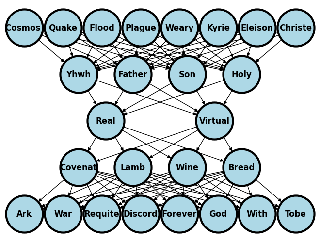
468. self-criticism#
Show code cell source
import networkx as nx
import matplotlib.pyplot as plt
import numpy as np
import sklearn as skl

#plt.figure(figsize=[2, 2])
G = nx.DiGraph()
G.add_node("Cosmos ",  pos = (0, 5) )
G.add_node("Quake",  pos = (1, 5) )
G.add_node("Flood",  pos = (2, 5) )
G.add_node("Plague",  pos = (3, 5) )
G.add_node("Weary",  pos = (4, 5) )
G.add_node("Kyrie",  pos = (5, 5) )
G.add_node("Eleison",  pos = (6, 5) )
G.add_node("Christe",  pos = (7, 5) )

G.add_node("Yhwh",  pos = (1.4, 4) )
G.add_node("Father",  pos = (2.8, 4) )
G.add_node("Son",  pos = (4.2, 4) )
G.add_node("Holy",  pos = (5.6, 4) )

G.add_node("Physical",  pos = (2.1, 3) )
G.add_node("Metaphys",  pos = (4.9, 3) )

G.add_node("Covenat",  pos = (1.4, 2) )
G.add_node("Lamb",  pos = (2.8, 2) )
G.add_node("Wine",  pos = (4.2, 2) )
G.add_node("Bread",  pos = (5.6, 2) )


G.add_node("Ark",  pos = (0, 1) )
G.add_node("War",  pos = (1, 1) )
G.add_node("Requite",  pos = (2, 1) )
G.add_node("Discord",  pos = (3, 1) )
G.add_node("Forever",  pos = (4, 1) )
G.add_node("God",  pos = (5, 1) )
G.add_node("With",  pos = (6, 1) )
G.add_node("Tobe",  pos = (7, 1) )

G.add_edges_from([ ("Cosmos ", "Yhwh"),  ("Cosmos ", "Father"),  ("Cosmos ", "Son"),  ("Cosmos ", "Holy")])
G.add_edges_from([ ("Quake", "Yhwh"),  ("Quake", "Father"),  ("Quake", "Son"),  ("Quake", "Holy")])
G.add_edges_from([ ("Flood", "Yhwh"),  ("Flood", "Father"),  ("Flood", "Son"),  ("Flood", "Holy")])
G.add_edges_from([ ("Plague", "Yhwh"),  ("Plague", "Father"),  ("Plague", "Son"),  ("Plague", "Holy")])
G.add_edges_from([ ("Weary", "Yhwh"),  ("Weary", "Father"),  ("Weary", "Son"),  ("Weary", "Holy")])
G.add_edges_from([ ("Kyrie", "Yhwh"),  ("Kyrie", "Father"),  ("Kyrie", "Son"),  ("Kyrie", "Holy")])
G.add_edges_from([ ("Eleison", "Yhwh"),  ("Eleison", "Father"),  ("Eleison", "Son"),  ("Eleison", "Holy")])
G.add_edges_from([ ("Christe", "Yhwh"),  ("Christe", "Father"),  ("Christe", "Son"),  ("Christe", "Holy")])

G.add_edges_from([ ("Yhwh", "Physical"),  ("Yhwh", "Metaphys")])
G.add_edges_from([ ("Father", "Physical"),  ("Father", "Metaphys")])
G.add_edges_from([ ("Son", "Physical"),  ("Son", "Metaphys")])
G.add_edges_from([ ("Holy", "Physical"),  ("Holy", "Metaphys")])


G.add_edges_from([ ("Physical", "Covenat"),  ("Physical", "Lamb"),  ("Physical", "Wine"),  ("Physical", "Bread")])
G.add_edges_from([ ("Metaphys", "Covenat"),  ("Metaphys", "Lamb"),  ("Metaphys", "Wine"),  ("Metaphys", "Bread")])

G.add_edges_from([ ("Covenat", "Ark"),  ("Covenat", "War"),  ("Covenat", "Requite"),  ("Covenat", "Discord")])
G.add_edges_from([ ("Covenat", "Forever"),  ("Covenat", "God"),  ("Covenat", "With"),  ("Covenat", "Tobe")])
G.add_edges_from([ ("Lamb", "Ark"),  ("Lamb", "War"),  ("Lamb", "Requite"),  ("Lamb", "Discord")])
G.add_edges_from([ ("Lamb", "Forever"),  ("Lamb", "God"),  ("Lamb", "With"),  ("Lamb", "Tobe")])
G.add_edges_from([ ("Wine", "Ark"),  ("Wine", "War"),  ("Wine", "Requite"),  ("Wine", "Discord")])
G.add_edges_from([ ("Wine", "Forever"),  ("Wine", "God"),  ("Wine", "With"),  ("Wine", "Tobe")])
G.add_edges_from([ ("Bread", "Ark"),  ("Bread", "War"),  ("Bread", "Requite"),  ("Bread", "Discord")])
G.add_edges_from([ ("Bread", "Forever"),  ("Bread", "God"),  ("Bread", "With"),  ("Bread", "Tobe")])


#G.add_edges_from([("H11", "H21"), ("H11", "H22"), ("H12", "H21"), ("H12", "H22")])
#G.add_edges_from([("H21", "Y"), ("H22", "Y")])
nx.draw(G,
        nx.get_node_attributes(G, 'pos'),
        with_labels=True,
        font_weight='bold',
        node_size = 3000,
        node_color = "lightblue",
        linewidths = 3)
ax= plt.gca()
ax.collections[0].set_edgecolor("#000000")
ax.set_xlim([-.5, 7.5])
ax.set_ylim([.5, 5.5])
plt.show()
Come unto me, all ye that labour and are heavy laden, and I will give you rest
– Matthew 11:28
467. babyface#
babyface
mmmhh
468. 2pac#
street 6:28/12:27
court
forgive?
i was like let’s have a charity match and give it to the kids.
and they were like no, we want him to do jail-time (deny the kids an opportunity, because… vindictive). that’s what they told the judge.
sort of echo’s a trump vs. letterman exchange
Show code cell source
import networkx as nx
import matplotlib.pyplot as plt
import numpy as np
import sklearn as skl

#plt.figure(figsize=[2, 2])
G = nx.DiGraph()
G.add_node("Cosmos ",  pos = (0, 5) )
G.add_node("Quake",  pos = (1, 5) )
G.add_node("Flood",  pos = (2, 5) )
G.add_node("Plague",  pos = (3, 5) )
G.add_node("Weary",  pos = (4, 5) )
G.add_node("Kyrie",  pos = (5, 5) )
G.add_node("Eleison",  pos = (6, 5) )
G.add_node("Christe",  pos = (7, 5) )

G.add_node("Yhwh",  pos = (1.4, 4) )
G.add_node("Father",  pos = (2.8, 4) )
G.add_node("Son",  pos = (4.2, 4) )
G.add_node("Holy",  pos = (5.6, 4) )

G.add_node("Street",  pos = (2.1, 3) )
G.add_node("Court",  pos = (4.9, 3) )

G.add_node("Covenat",  pos = (1.4, 2) )
G.add_node("Lamb",  pos = (2.8, 2) )
G.add_node("Wine",  pos = (4.2, 2) )
G.add_node("Bread",  pos = (5.6, 2) )


G.add_node("Ark",  pos = (0, 1) )
G.add_node("War",  pos = (1, 1) )
G.add_node("Requite",  pos = (2, 1) )
G.add_node("Discord",  pos = (3, 1) )
G.add_node("Forever",  pos = (4, 1) )
G.add_node("God",  pos = (5, 1) )
G.add_node("With",  pos = (6, 1) )
G.add_node("Tobe",  pos = (7, 1) )

G.add_edges_from([ ("Cosmos ", "Yhwh"),  ("Cosmos ", "Father"),  ("Cosmos ", "Son"),  ("Cosmos ", "Holy")])
G.add_edges_from([ ("Quake", "Yhwh"),  ("Quake", "Father"),  ("Quake", "Son"),  ("Quake", "Holy")])
G.add_edges_from([ ("Flood", "Yhwh"),  ("Flood", "Father"),  ("Flood", "Son"),  ("Flood", "Holy")])
G.add_edges_from([ ("Plague", "Yhwh"),  ("Plague", "Father"),  ("Plague", "Son"),  ("Plague", "Holy")])
G.add_edges_from([ ("Weary", "Yhwh"),  ("Weary", "Father"),  ("Weary", "Son"),  ("Weary", "Holy")])
G.add_edges_from([ ("Kyrie", "Yhwh"),  ("Kyrie", "Father"),  ("Kyrie", "Son"),  ("Kyrie", "Holy")])
G.add_edges_from([ ("Eleison", "Yhwh"),  ("Eleison", "Father"),  ("Eleison", "Son"),  ("Eleison", "Holy")])
G.add_edges_from([ ("Christe", "Yhwh"),  ("Christe", "Father"),  ("Christe", "Son"),  ("Christe", "Holy")])

G.add_edges_from([ ("Yhwh", "Street"),  ("Yhwh", "Court")])
G.add_edges_from([ ("Father", "Street"),  ("Father", "Court")])
G.add_edges_from([ ("Son", "Street"),  ("Son", "Court")])
G.add_edges_from([ ("Holy", "Street"),  ("Holy", "Court")])


G.add_edges_from([ ("Street", "Covenat"),  ("Street", "Lamb"),  ("Street", "Wine"),  ("Street", "Bread")])
G.add_edges_from([ ("Court", "Covenat"),  ("Court", "Lamb"),  ("Court", "Wine"),  ("Court", "Bread")])

G.add_edges_from([ ("Covenat", "Ark"),  ("Covenat", "War"),  ("Covenat", "Requite"),  ("Covenat", "Discord")])
G.add_edges_from([ ("Covenat", "Forever"),  ("Covenat", "God"),  ("Covenat", "With"),  ("Covenat", "Tobe")])
G.add_edges_from([ ("Lamb", "Ark"),  ("Lamb", "War"),  ("Lamb", "Requite"),  ("Lamb", "Discord")])
G.add_edges_from([ ("Lamb", "Forever"),  ("Lamb", "God"),  ("Lamb", "With"),  ("Lamb", "Tobe")])
G.add_edges_from([ ("Wine", "Ark"),  ("Wine", "War"),  ("Wine", "Requite"),  ("Wine", "Discord")])
G.add_edges_from([ ("Wine", "Forever"),  ("Wine", "God"),  ("Wine", "With"),  ("Wine", "Tobe")])
G.add_edges_from([ ("Bread", "Ark"),  ("Bread", "War"),  ("Bread", "Requite"),  ("Bread", "Discord")])
G.add_edges_from([ ("Bread", "Forever"),  ("Bread", "God"),  ("Bread", "With"),  ("Bread", "Tobe")])


#G.add_edges_from([("H11", "H21"), ("H11", "H22"), ("H12", "H21"), ("H12", "H22")])
#G.add_edges_from([("H21", "Y"), ("H22", "Y")])
nx.draw(G,
        nx.get_node_attributes(G, 'pos'),
        with_labels=True,
        font_weight='bold',
        node_size = 3000,
        node_color = "lightblue",
        linewidths = 3)
ax= plt.gca()
ax.collections[0].set_edgecolor("#000000")
ax.set_xlim([-.5, 7.5])
ax.set_ylim([.5, 5.5])
plt.show()
469. brando#
life/art
we’re all actors
470. bebe&cece#
i’m lost without you
back up singers!
angie, debbie, whitney
471. autoencoder#
dream it
encode/chase it
tame it
reproduce it
472. arsenio#
probably what destroyed his career
this very specific interview
which brings to mind a couple of things:
supervised learning (fellow humans label what is good & bad: genealogy of morality)
unsupervised learning (human-designed algorithm uncovers, clusters, heretofore unbeknownst relationships)
adaptive learning (an algorithm that may keep on shocking its creators, since it goes beyond what was dreamed of by the engineers who wrote it)
473. vanilla#
ice
was
i’d like to give a shout out to my …
474. doppelgänger#
victoria monét
betty ndagijimana
there’s a je ne sais quoi
06/11/2023#
475. adversarial#
networks
challenge vs. skill
to infinity & beyond work-/lifeflow
476. linda#
ko, he said to the woman in labor
her baby was crowning at this point
but he was, gloved, examining another in labor
likewise, he told anxious graduate students:
don’t worry about grades and just focus on learning
where’s the empathy in all of this?
yes, i was trying to assure them that this adversarial network, wherein i’m the challenger, will present low-to-mid level challenges; just enough to nurture their budding skills
but what does that even mean? how is a challenge calibrated? well, the students didn’t buy it and so they wrote scathing reviews - courseeval is a necessary prerequisite for access to their grades
school response rate was 84%, epidemiology 89%, my course 92% (never at any point did i mention course eval). anxious, upset people are quite motivated to write reviews; its the negative emotion that drives us and our memories beyond
477. todolistspecial#
get reviews from 2021-2023
respond to each + & - in updates
iterate this summer, overhaul next spring
478. notes#
here are a few highlights. but first, remember that difficult classes do not always produce low student satisfaction. there is evidence that students value a challenge if they feel they have been given the tools to meet that challenge
478.1#
this was 600.71 with 110 taking it for a grade. generally, course and school term mean were about the same for all metrics. response rates were 95% (course), 91% (epi), 88% (school)
strengths
volume of material can’t be taught anywhere else
resources: lecture, do file (well annotated), lab
feedback on hw was extremely important
assignments were
challengingbut rewarding, leveraged in other classes
weaknesses
not
engaging: just commandsconcepts not developed
a lot covered in a short time
too much time answering students (should do this in office hours)
students watch videos of coding: then class is problem solving
grading timeliness could be improved
provide answer keys!
discordance between lectures and hws
feels like a 3cr class
boring to teach coding, and ta’s often lacked knowledge
two hours is way too much and dull if command after command
opportunities
change to 3cr
or easier hws
split 2hr: in-class ex
transparency
+ early release of grading rubrics + describe subjective & objective elements of rubric
threats
students who had a bad experience and will strongly advise against this class
it comes in the fourth term; too little, too late?
random
478.2#
this was 700.71 with 10 students all for a grade. response rates were 100%, 89%, 84%
👎
course organization
assessment of learning
spent 10hrs/week vs. 6 for epi/school
👍
expanded knowledge
achieved objectives
478.3#
and the 600.01 class had a relative response rate of 92% (course n=60), 89% (epi n=703), and 84% (school n=8492)
👎
course organization
assessment of learning
primary instructor
👍
achieved objectives
expanded knowledge
improved
skills
details
poorly designed website
important items intentionally hiddenlectures felt like a stream of consciousness
mockery of students concerned about grades
no transparency in grading or rubric
chapters with plain titles and objectives
a complaint about 10% off for
if 0 {conditionaldescribed as meaningless annotation in hw1
the emphasis on formatting in grading hw was too much
professor needs remediation on learning thoery & professionalism
the class felt very disorganized, but i know this is due to the reorganization of the course. i like the idea of using git hub and think it will be useful once the pages are more organized - maybe having a centralized page with all the necessary links and schedules. the grading was also a little confusing. I think a rubric up front would be so helpful so students know what to prioritize
478.4#
600.79 had 11/18 (61%) response rate compared with 75% (epi n=493) & 76% (school n=2077)
👎
below average for feedback
ta’s
👍
course above school-term mean for:
instructor
organization
assessment of learning
expanded my knowledge
improved my skill
focused & organized instruction & content
skills taught exactly what you need in the real world work place
dofiles, lecture notes, annotation will be great resources even in the future
very focused on high yield topics. great course resources
i think it helps to have a basic statistics background and maybe some basic knowledge of how stata operates (what a do file is, how to import a dataset or use a data set, etc).
i think the most helpful thing about the course was that dr. xxx went over student’s code and their challenges during the class. it helped us know what the fault in our codes was at the spot. i think it helped the whole class. there was also a lot of repetition in class which consolidated the topic.
for course content, it might be helpful to have messy data to work with - in the real world, datasets and everyday functions aren’t as clear cut as those introduced in class.
Feedback on assignments could have been a little faster but there was plenty of flexibility built in to account for this.
479. negative#
is mnemonic
positive less so
how to weigh each!
481. brando#
all the worlds a stage…
marlo brando said it best:
we are all actors:
when someone asks how are you?
if you see someone you wish to criticize!
our responses are a mode of acting
because we sort of know at least something about our audience, even when they’re strangers:
skilllevel of our audience comes to mindare they motivated to advance their skills?
or tolerate our
challenges?so, we titrate the challenges we bring along in every encounter
from the outset we recognize and offer a hierarchy of challenges based on 1, 2, 3 above
but its an idea to initially focus on the lowest challenge and show pathway to higher challenges
that is, if our audience are “game”, if they’re a good sport
06/13/2023#
482. sinusitis#
last 15 years
exacerbated in 03/2016
and worst-ever from 2022-2023
these were periods of daily swimming
usually 1-2 miles (close to 2 hours a day)
i’d call it swimmers sinusitis
sounds like i have a cold to those i speak with on the phone
time to schedule an appointment with ent surgeon
483. stata#
system
native (stata application & support files, e.g. ado files)
third-party (support files, typically ado files)
your future role (as students in this class; i.e., ado files that you’ll write and install)
user
known
you
me
teaching assistants
collaborators
unknown
anticipate (i.e., empathize with different kinds of users)
share code (e.g. on github)
care (i.e., user-frienly code with annotation)
installation
local
MacOSX
Unix
Windows
remote
Desktop
Windows
Cluster
Unix/Terminal
local
-
file
edit
data
graphics
statistics
user
window
command ⌘ 1
results ⌘ 2
history ⌘ 3
variables ⌘ 4
properties ⌘ 5
graph ⌘ 6
viewer ⌘ 7
editor ⌘ 8
do-file ⌘ 9
manager ⌘ 10
help
command
the very first
legitimateword you type into the command window or on a line of code in a do fileon my computer it is always rendered blue in color if its a native Stata command
if developed by a third-party then it is white and may not work if you share your do file with others
your collaborators, ta’s, and instructors must be warned to first install the third-party program
syntax
the arrangement of words after a stata command
create well-formed instructions in stata (i.e.,
the syntax of Stata)other terms or synonyms include
code,stata code,code snippet
input
menu (outputs command and syntax in results)
do files (script with a series of commands)
ado files (script with a program or series of programs)
output
numeric:
byte
double
long
string
plain text
file paths
urls
embed
consol window
log file
excel file
word doc
html doc
publish
self (e.g. github)
journal (e.g. jama)
-
remote
desktop: a few of you may use this, which presents unique challenges for this class
terminal: unlikely that any of you will be using this, since its for advanced programmers
menu
file > example datasets > lifeexp.dta > use
sysuse lifeexp.dta
webuse sysuse lifeexp.dta
command
import data into stata
webuse lifeexp, clear
. webuse lifeexp, clear
(Life expectancy, 1998)

.
explore the imported data
display c(N)
display c(k)
describe
. display c(N)
68

. display c(k)
6

. describe

Contains data from https://www.stata-press.com/data/r18/lifeexp.dta
Observations:            68                  Life expectancy, 1998
Variables:                6                  26 Mar 2022 09:40
(_dta has notes)

Variable      Storage   Display    Value
name         type    format    label      Variable label

region          byte    %16.0g     region     Region
country         str28   %28s                  Country
popgrowth       float   %9.0g               * Avg. annual % growth
lexp            byte    %9.0g               * Life expectancy at birth
gnppc           float   %9.0g               * GNP per capita
safewater       byte    %9.0g               * Safe water
* indicated variables have	notes

Sorted by:

.
perform basic analysis
webuse lifeexp, clear
describe
encode country, gen(Country)
twoway scatter lexp Country, xscale(off)
graph export lexp_bycountry.png, replace
. webuse lifeexp, clear
(Life expectancy, 1998)

. describe

Contains data from https://www.stata-press.com/data/r18/lifeexp.dta
Observations:            68                  Life expectancy, 1998
Variables:                6                  26 Mar 2022 09:40
(_dta has notes)

Variable      Storage   Display    Value
name         type    format    label      Variable label

region          byte    %16.0g     region     Region
country         str28   %28s                  Country
popgrowth       float   %9.0g               * Avg. annual % growth
lexp            byte    %9.0g               * Life expectancy at birth
gnppc           float   %9.0g               * GNP per capita
safewater       byte    %9.0g               * Safe water
* indicated variables have	notes

Sorted by:

. encode country, gen(Country)

. twoway scatter lexp Country, xscale(off)

. graph export lexp_bycountry.png, replace
file /Users/d/Desktop/lexp_bycountry.png saved as PNG format

.
end of do-file

.

do file
importing data
exploring data
analyzing data
outputing results
ado file
basis of stata commands
innate or third-party
we shall be learning to write basic programs (i.e.
stata programming)
etc
gradually build these concepts beginning with sys/user:
system-defined
constantsor c-class commands
creturn list
. creturn list

System values


c(current_date) = "13 Jun 2023"
c(current_time) = "10:43:51"
c(rmsg_time) = 0	(seconds, from set rmsg)

c(stata_version) = 18
c(version) = 18	(version)
c(userversion) = 18	(version)
c(dyndoc_version) = 2	(dyndoc)

c(born_date) = "15 May 2023"
c(edition) = "BE"
c(edition_real) = "SE"
c(bit) = 64
c(SE) = 1
c(MP) = 0
c(processors) = 1	(Stata/MP, set processors)
c(processors_lic) = 1
c(processors_mach) = .
c(processors_max) = 1
c(mode) = ""
c(console) = ""

c(os) = "MacOSX"
c(osdtl) = "13.4.0"
c(hostname) = "Poseidon.local"
c(machine_type) = "Macintosh (Intel .."
c(byteorder) = "lohi"
c(username) = "d"


Directories and paths


c(sysdir_stata) = "/Applications/Sta.."	(sysdir)
c(sysdir_base) = "/Applications/Sta.."	(sysdir)
c(sysdir_site) = "/Applications/Sta.."	(sysdir)
c(sysdir_plus) = "/Users/d/Library/.."	(sysdir)
c(sysdir_personal) = "/Users/d/Document.."	(sysdir)
c(sysdir_oldplace) = "~/ado/"	(sysdir)
c(tmpdir) = "/var/folders/sx/f.."

c(adopath) = "BASE;SITE;.;PERSO.."	(adopath)
c(pwd) = "/Users/d/Desktop"	(cd)
c(dirsep) = "/"


System limits


c(max_N_theory) = 2147483620
c(max_k_theory) = 5000	(set maxvar)
c(max_width_theory) = 1048576	(set maxvar)

c(max_matdim) = 11000

c(max_it_cvars) = 64
c(max_it_fvars) = 8

c(max_macrolen) = 4227143
c(macrolen) = 645200	(set maxvar)
c(charlen) = 67783
c(max_cmdlen) = 4227159
c(cmdlen) = 645216	(set maxvar)
c(namelenbyte) = 128
c(namelenchar) = 32
c(eqlen) = 1337


Numerical and string limits


c(mindouble) = -8.9884656743e+307
c(maxdouble) = 8.9884656743e+307
c(epsdouble) = 2.22044604925e-16
c(smallestdouble) = 2.2250738585e-308

c(minfloat) = -1.70141173319e+38
c(maxfloat) = 1.70141173319e+38
c(epsfloat) = 1.19209289551e-07

c(minlong) = -2147483647
c(maxlong) = 2147483620

c(minint) = -32767
c(maxint) = 32740

c(minbyte) = -127
c(maxbyte) = 100

c(maxstrvarlen) = 2045
c(maxstrlvarlen) = 2000000000
c(maxvlabellen) = 32000


Current dataset


c(frame) = "default"
c(N) = 68
c(k) = 6
c(width) = 39
c(changed) = 0
c(filename) = "https://www.stata.."
c(filedate) = "26 Mar 2022 09:40"


Memory settings


c(memory) = 33554432
c(maxvar) = 5000	(set maxvar)
c(niceness) = 5	(set niceness)
c(min_memory) = 0	(set min_memory)
c(max_memory) = .	(set max_memory)
c(segmentsize) = 33554432	(set segmentsize)
c(adosize) = 1000	(set adosize)


Output settings


c(more) = "off"	(set more)
c(rmsg) = "off"	(set rmsg)
c(dp) = "period"	(set dp)
c(linesize) = 196	(set linesize)
c(pagesize) = 61	(set pagesize)
c(logtype) = "smcl"	(set logtype)
c(logmsg) = "on"	(set logmsg)
c(noisily) = 1
c(notifyuser) = "on"	(set notifyuser)
c(playsnd) = "off"	(set playsnd)
c(include_bitmap) = "on"	(set include_bitmap)

c(iterlog) = "on"	(set iterlog)

c(level) = 95	(set level)
c(clevel) = 95	(set clevel)

c(showbaselevels) = ""	(set showbaselevels)
c(showemptycells) = ""	(set showemptycells)
c(showomitted) = ""	(set showomitted)
c(fvlabel) = "on"	(set fvlabel)
c(fvwrap) = 1	(set fvwrap)
c(fvwrapon) = "word"	(set fvwrapon)
c(lstretch) = ""	(set lstretch)

c(cformat) = ""	(set cformat)
c(sformat) = ""	(set sformat)
c(pformat) = ""	(set pformat)

c(coeftabresults) = "on"	(set coeftabresults)
c(dots) = "on"	(set dots)

c(collect_label) = "default"	(set collect_label)
c(collect_style) = "default"	(set collect_style)
c(table_style) = "table"	(set table_style)
c(etable_style) = "etable"	(set etable_style)
c(dtable_style) = "dtable"	(set dtable_style)
c(collect_warn) = "on"	(set collect_warn)


Interface settings


c(reventries) = 5000	(set reventries)
c(revkeyboard) = "on"	(set revkeyboard)
c(varkeyboard) = "on"	(set varkeyboard)
c(smoothfonts) = "on"	(set smoothfonts)
c(linegap) = 1	(set linegap)
c(scrollbufsize) = 204800	(set scrollbufsize)
c(maxdb) = 50	(set maxdb)


Graphics settings


c(graphics) = "on"	(set graphics)
c(scheme) = "stcolor"	(set scheme)
c(printcolor) = "asis"	(set printcolor)
c(copycolor) = "asis"	(set copycolor)
c(maxbezierpath) = 0	(set maxbezierpath)
c(min_graphsize) = 1	(region_options)
c(max_graphsize) = 100	(region_options)


Network settings


c(httpproxy) = "off"	(set httpproxy)
c(httpproxyhost) = ""	(set httpproxyhost)
c(httpproxyport) = 80	(set httpproxyport)

c(httpproxyauth) = "off"	(set httpproxyauth)
c(httpproxyuser) = ""	(set httpproxyuser)
c(httpproxypw) = ""	(set httpproxypw)


Update settings


c(update_query) = "on"	(set update_query)
c(update_interval) = 7	(set update_interval)
c(update_prompt) = "on"	(set update_prompt)


Trace (program debugging) settings


c(trace) = "off"	(set trace)
c(tracedepth) = 32000	(set tracedepth)
c(tracesep) = "on"	(set tracesep)
c(traceindent) = "on"	(set traceindent)
c(traceexpand) = "on"	(set traceexpand)
c(tracenumber) = "off"	(set tracenumber)
c(tracehilite) = ""	(set tracehilite)


Mata settings


c(matastrict) = "off"	(set matastrict)
c(matalnum) = "off"	(set matalnum)
c(mataoptimize) = "on"	(set mataoptimize)
c(matafavor) = "space"	(set matafavor)
c(matacache) = 2000	(set matacache)
c(matalibs) = "lmatabase;lmatamc.."	(set matalibs)
c(matamofirst) = "off"	(set matamofirst)
c(matasolvetol) = .	(set matasolvetol)


Java settings


c(java_heapmax) = "4096m"	(set java_heapmax)
c(java_home) = "/Applications/Sta.."	(set java_home)


LAPACK settings


c(lapack_mkl) = "on"	(set lapack_mkl)
c(lapack_mkl_cnr) = "default"	(set lapack_mkl_cnr)


putdocx settings


c(docx_hardbreak) = "off"	(set docx_hardbreak)
c(docx_paramode) = "off"	(set docx_paramode)


Python settings


c(python_exec) = ""	(set python_exec)
c(python_userpath) = ""	(set python_userpath)


RNG settings


c(rng) = "default"	(set rng)
c(rng_current) = "mt64"
c(rngstate) = "XAA00000000000000.."	(set rngstate)
c(rngseed_mt64s) = 123456789
c(rngstream) = 1	(set rngstream)


sort settings


c(sortmethod) = "default"	(set sortmethod)
c(sort_current) = "fsort"
c(sortrngstate) = "775915113XZA11221.."	(set sortrngstate)


Unicode settings


c(locale_ui) = "en_US"	(set locale_ui)
c(locale_functions) = "en_US"	(set locale_functions)
c(locale_icudflt) = "en_US"	(unicode locale)


Other settings


c(type) = "float"	(set type)
c(maxiter) = 300	(set maxiter)
c(searchdefault) = "all"	(set searchdefault)
c(varabbrev) = "on"	(set varabbrev)
c(emptycells) = "keep"	(set emptycells)
c(fvtrack) = "term"	(set fvtrack)
c(fvbase) = "on"	(set fvbase)
c(odbcmgr) = "iodbc"	(set odbcmgr)
c(odbcdriver) = "unicode"	(set odbcdriver)
c(fredkey) = ""	(set fredkey)
c(collect_double) = "on"	(set collect_double)
c(dtascomplevel) = 1	(set dtascomplevel)


Other system values


c(pi) = 3.141592653589793
c(alpha) = "a b c d e f g h i.."
c(ALPHA) = "A B C D E F G H I.."
c(Mons) = "Jan Feb Mar Apr M.."
c(Months) = "January February .."
c(Wdays) = "Sun Mon Tue Wed T.."
c(Weekdays) = "Sunday Monday Tue.."
c(obs_t) = "byte"
c(rc) = 0	(capture)


.
user-defined
returnor r-class commands
webuse lifeexp, clear
sum lexp
return list
. webuse lifeexp, clear
(Life expectancy, 1998)

. sum lexp

Variable         Obs	Mean    Std. dev.	Min	Max

lexp          68	72.27941    4.715315	54	79

. return list

scalars:
r(N) =	68
r(sum_w) =	68
r(mean) =	72.27941176470588
r(Var) =	22.23419666374012
r(sd) =	4.715315118180345
r(min) =	54
r(max) =	79
r(sum) =	4915

.
stata-estimated
ereturnor e-class commands
regress lexp safewater
. regress lexp safewater

Source        SS           df       MS      Number of obs   =	40
__________________________________________  F(1, 38)        =	83.97
   Model   710.45849       1  710.45849     Prob > F        =	0.0000
Residual   321.51651      38    8.46096078  R-squared       =	0.6884
__________________________________________  Adj R-squared   =	0.6802
Total     1031.975        39   26.4608974   Root MSE        =	2.9088
_________________________________________________________________________
_________________________________________________________________________
     lexp  Coefficient  Std. err.      t    P>t     [95% conf.	interval]
_________________________________________________________________________
safewater      .238561   .0260339    9.16   0.000       .185858	  .291264
    _cons    53.32051   2.033866    26.22   0.000     49.20316	57.43785


. ereturn list

scalars:
e(N) =  40
e(df_m) =  1
e(df_r) =  38
e(F) =  83.96900881198023
e(r2) =  .6884454471661862
e(rmse) =  2.908773071338512
e(mss) =  710.458490339325
e(rss) =  321.516509660675
e(r2_a) =  .6802466431442438
e(ll) =  -98.44093013263662
e(ll_0) =  -121.7645466647458
e(rank) =  2

macros:
e(cmdline) : "regress lexp safewater"
e(title) : "Linear regression"
e(marginsok) : "XB default"
e(vce) : "ols"
e(depvar) : "lexp"
e(cmd) : "regress"
e(properties) : "b V"
e(predict) : "regres_p"
e(model) : "ols"
e(estat_cmd) : "regress_estat"

matrices:
e(b) :  1 x 2
e(V) :  2 x 2
e(beta) :  1 x 1

functions:
e(sample)

.
Baltimore Crab 🦀#
Show code cell source
import networkx as nx
import matplotlib.pyplot as plt
#import numpy as np
#import sklearn as skl
#

#plt.figure(figsize=[2, 2])
G = nx.DiGraph()
G.add_node("user",  pos = (550,500) )
G.add_node("system",  pos = (-550,500) )
G.add_node("program",  pos = (-2000, 960) )
G.add_node("syntax",  pos = (2000, 950) )
G.add_node("ado", pos = (-3000, 550) )
G.add_node("do", pos = (3000, 550) )
G.add_node("command", pos = (-1900, 150) )
G.add_node("queue", pos = (1900, 150) )
G.add_node("output", pos = (0,0))
G.add_node("dta", pos = (0, -475))
G.add_node("log", pos = (-1900, -475))
G.add_node("excel", pos = (-4000, -475))
G.add_node("word", pos = (1900, -475))
G.add_node("html", pos = (4000, -475))
G.add_node("publish", pos = (0, -950))
G.add_edges_from([ ("program","ado"), ("syntax", "do")])
G.add_edges_from([("ado", "command"), ("do", "queue") ])
G.add_edges_from([("command", "output"), ("queue", "output"),("output","excel"),("output","word"),("output","html")])
G.add_edges_from([("output","dta"),("output","log")])
G.add_edges_from([("dta","publish"),("log","publish"),("excel","publish"),("word","publish"),("html","publish")])
nx.draw(G,
        nx.get_node_attributes(G, 'pos'),
        with_labels=True,
        font_weight='bold',
        node_size = 4500,
        node_color = "lightblue",
        linewidths = 3)
ax= plt.gca()
ax.collections[0].set_edgecolor("#000000")
ax.set_xlim([-5000, 5000])
ax.set_ylim([-1000, 1000])
plt.show()
484. linguo#
We are going to distinguish between two fundamental things in this class:
the system; and,
the user
The system is the Stata application and its a simple noun. It is not STATA, which gives the impression of being an acronym. I presume you’ve all installed Stata onto your local machines. If not I presume you’ll be doing so very soon or you will be remotely accessing it. The user is you, me, the teaching assistants, any collaborator, or stranger.
Soon, we will begin to write Stata programs and install them into the system folders. Then, it will be helpful to think of your role at as part of the system. In your new role as system, it will be helpful to anticipate the needs of the known and unknown future user of your program. This calls for empathy (anticipating user needs), sharing (your code with others), and caring (that its user-friendly).
485. chatGPT#
485.1 basic#
Remember this basic analysis?
webuse lifeexp, clear
describe
encode country, gen(Country)
sort lexp
twoway scatter lexp Country, xscale(off)
graph export lexp_bycountry.png, replace
. sort lexp

. gen Country=_n

. twoway scatter lexp Country

. graph export lexp_bycountry.png, replace
file /Users/d/Desktop/lexp_bycountry.png saved as PNG format

.
485.2 improve#
What if you wish to improve this ouput? How may you make it more informative? Ever considered chatGPT?

Let’s implement what chatGPT has suggested.
webuse lifeexp, clear
encode country, gen(Country)
twoway (scatter lexp Country, mlabel(Country) xscale(off))
graph export lexp_bycountry_withlabels.png, replace
. webuse lifeexp, clear
(Life expectancy, 1998)

. encode country, gen(Country)

. twoway (scatter lexp Country, mlabel(Country)) xscale(off)

. graph export lexp_bycountry_withlabels.png
file /Users/d/Desktop/lexp_bycountry_withlabels.png	saved as PNG format

.

485.3 order#
Now lets sort by life expectancy to create a semblance of order. This cost me the better part of 10 hours. I’ve now incorporated subinstr into my arsenal. That was the key issue!
//chatGPT+vincent
cls
clear
webuse lifeexp
sort lexp
g rank=_n
tostring rank, replace
g dx=rank+"="+country
replace dx=substr(dx,1,31)
drop country rank
replace dx=subinstr(dx," ","",.)
replace dx = subinstr(dx, "\", "", .)
replace dx = subinstr(dx, "(", "", .)
replace dx = subinstr(dx, ")", "", .)
replace dx = subinstr(dx, ",", "", .)
replace dx = subinstr(dx, "/", "", .)

levelsof dx, local(dx_helper)
foreach i in `dx_helper' {
    tokenize `"`i'"', p("=")
    //local label_value: di "`1'"
    //local label_text: di "`3'"
	local label_string: di `"  `label_string' `1' "`3'"    "'
    //local label_string: di "   `label_string'" `label_value' `"`label_text'"'  "
	//local label_string: di "`label_string' `" `label_value' `"`label_text'"'"

	di `label_string'
}

global chatgpt: di `label_string'
di "$chatgpt"
//macro list
capture label drop dx
label define dx `label_string'
split dx, p("=")
destring dx1, replace
label values dx1 dx
noi tab dx1

twoway scatter lexp dx1, mlabel(dx1) xscale(off)
graph export lexp_bycountry_withlabels_sort.png, replace
. clear

. webuse lifeexp
(Life expectancy, 1998)

. sort lexp

. g rank=_n

. tostring rank, replace
rank was float now str2

. g dx=rank+"="+country

. replace dx=substr(dx,1,31)
(0 real changes made)

. drop country rank

. replace dx=subinstr(dx," ","",.)
(13 real changes made)

. replace dx = subinstr(dx, "\", "", .)
(0 real changes made)

. replace dx = subinstr(dx, "(", "", .)
(1 real change made)

. replace dx = subinstr(dx, ")", "", .)
(1 real change made)

. replace dx = subinstr(dx, ",", "", .)
(1 real change made)

. replace dx = subinstr(dx, "/", "", .)
(1 real change made)

.
. qui levelsof dx, local(dx_helper)

. foreach i in `dx_helper' {
2.     tokenize `"`i'"', p("=")
3.     //local label_value: di "`1'"
.     //local label_text: di "`3'"
.         local label_string: di `"  `label_string' `1' "`3'"    "'
4.     //local label_string: di "   `label_string'" `label_value' `"`label_text'"'	"
.         //local label_string: di "`label_string' `" `label_value' `"`label_text'"'"
.
.         //di `label_string'
. }

.
. global chatgpt: di `label_string'

. //di "$chatgpt"
. //macro list
. capture label drop dx

. label define dx `label_string'

. split dx, p("=")
variables created as string:
dx1  dx2

. destring dx1, replace
dx1: all characters numeric; replaced as byte

. label values dx1 dx

. //noi tab dx1
.
. twoway scatter lexp dx1, mlabel(dx1) xscale(off)

. graph export lexp_bycountry_withlabels_sort.png, replace
file /Users/d/Desktop/lexp_bycountry_withlabels_sort.png saved as PNG format

.
.
.
end of do-file

.

485.4 legible#
cls
clear
webuse lifeexp
sort lexp
g rank=_n
tostring rank, replace
g dx=rank+"="+country
replace dx=substr(dx,1,31)
drop country rank
replace dx=subinstr(dx," ","",.)
replace dx = subinstr(dx, "\", "", .)
replace dx = subinstr(dx, "(", "", .)
replace dx = subinstr(dx, ")", "", .)
replace dx = subinstr(dx, ",", "", .)
replace dx = subinstr(dx, "/", "", .)

qui levelsof dx, local(dx_helper)
foreach i in `dx_helper' {
    tokenize `"`i'"', p("=")
	local label_string: di `"  `label_string' `1' "`3'"    "'
	//di `label_string'
}

global chatgpt: di `label_string'
//di "$chatgpt"
//macro list
capture label drop dx
label define dx `label_string'
split dx, p("=")
destring dx1, replace
label values dx1 dx
//noi tab dx1
#delimit ;
twoway scatter dx1 lexp, sort
   mlabel(dx1)
   yscale(off)
;
#delimit cr
graph export lexp_bycountry_withlabels_sort_horizontal.png, replace
. clear

. webuse lifeexp
(Life expectancy, 1998)

. sort lexp

. g rank=_n

. tostring rank, replace
rank was float now str2

. g dx=rank+"="+country

. replace dx=substr(dx,1,31)
(0 real changes made)

. drop country rank

. replace dx=subinstr(dx," ","",.)
(13 real changes made)

. replace dx = subinstr(dx, "\", "", .)
(0 real changes made)

. replace dx = subinstr(dx, "(", "", .)
(1 real change made)

. replace dx = subinstr(dx, ")", "", .)
(1 real change made)

. replace dx = subinstr(dx, ",", "", .)
(1 real change made)

. replace dx = subinstr(dx, "/", "", .)
(1 real change made)

.
. qui levelsof dx, local(dx_helper)

. foreach i in `dx_helper' {
  2.     tokenize `"`i'"', p("=")
  3.         local label_string: di `"  `label_string' `1' "`3'"    "'
  4.         //di `label_string'
. }

.
. global chatgpt: di `label_string'

. //di "$chatgpt"
. //macro list
. capture label drop dx

. label define dx `label_string'

. split dx, p("=")
variables created as string:
dx1  dx2

. destring dx1, replace
dx1: all characters numeric; replaced as byte

. label values dx1 dx

. //noi tab dx1
. #delimit ;
delimiter now ;
. twoway scatter dx1 lexp, sort
>    mlabel(dx1)
>    yscale(off)
> ;

. #delimit cr
delimiter now cr
. graph export lexp_bycountry_withlabels_sort_horizontal.png, replace
file /Users/d/Desktop/lexp_bycountry_withlabels_sort_horizontal.png saved as PNG format

.
end of do-file

.

485.5 stratified#
clear
webuse lifeexp
sort lexp
g rank=_n
tostring rank, replace
g dx=rank+"="+country
replace dx=substr(dx,1,31)
drop country rank
replace dx=subinstr(dx," ","",.)
replace dx = subinstr(dx, "\", "", .)
replace dx = subinstr(dx, "(", "", .)
replace dx = subinstr(dx, ")", "", .)
replace dx = subinstr(dx, ",", "", .)
replace dx = subinstr(dx, "/", "", .)

qui levelsof dx, local(dx_helper)
foreach i in `dx_helper' {
    tokenize `"`i'"', p("=")
	local label_string: di `"  `label_string' `1' "`3'"    "'
	//di `label_string'
}

global chatgpt: di `label_string'
//di "$chatgpt"
//macro list
capture label drop dx
label define dx `label_string'
split dx, p("=")
destring dx1, replace
label values dx1 dx
//noi tab dx1
#delimit ;
twoway (scatter dx1 lexp if region==1,
   sort
   mlabel(dx1)
   yscale(off)
   title("Europe & C. Asia")
   );
graph save lexp_bycountry1.gph, replace ;
twoway (scatter dx1 lexp if region==2,
   sort
   mlabel(dx1)
   yscale(off)
   title("North America")
   );
graph save lexp_bycountry2.gph, replace ;
twoway (scatter dx1 lexp if region==3,
   sort
   mlabel(dx1)
   yscale(off)
   title("South America")
   );
graph save lexp_bycountry3.gph, replace ;
graph combine
    lexp_bycountry1.gph
    lexp_bycountry2.gph
	lexp_bycountry3.gph,
	xcommon col(3);
#delimit cr
graph export lexp_bycountry_combine.png, replace
. clear

. webuse lifeexp
(Life expectancy, 1998)

. sort lexp

. g rank=_n

. tostring rank, replace
rank was float now str2

. g dx=rank+"="+country

. replace dx=substr(dx,1,31)
(0 real changes made)

. drop country rank

. replace dx=subinstr(dx," ","",.)
(13 real changes made)

. replace dx = subinstr(dx, "\", "", .)
(0 real changes made)

. replace dx = subinstr(dx, "(", "", .)
(1 real change made)

. replace dx = subinstr(dx, ")", "", .)
(1 real change made)

. replace dx = subinstr(dx, ",", "", .)
(1 real change made)

. replace dx = subinstr(dx, "/", "", .)
(1 real change made)

.
. qui levelsof dx, local(dx_helper)

. foreach i in `dx_helper' {
2.     tokenize `"`i'"', p("=")
3.         local label_string: di `"  `label_string'	`1' "`3'"    "'
4.         //di `label_string'
. }

.
. global chatgpt: di `label_string'

. //di "$chatgpt"
. //macro list
. capture label drop dx

. label define dx `label_string'

. split dx, p("=")
variables created as string:
dx1  dx2

. destring dx1, replace
dx1: all characters numeric; replaced as byte

. label values dx1 dx

. //noi tab dx1
. #delimit ;
delimiter now ;
. twoway (scatter dx1 lexp if region==1,
>    sort
>    mlabel(dx1)
>    yscale(off)
>    title("Europe & C. Asia")
>    );

.  graph save lexp_bycountry1.gph, replace ;
file lexp_bycountry1.gph saved

.  twoway (scatter dx1 lexp if region==2,
>    sort
>    mlabel(dx1)
>    yscale(off)
>    title("North America")
>    );

.  graph save lexp_bycountry2.gph, replace ;
file lexp_bycountry2.gph saved

.  twoway (scatter dx1 lexp if region==3,
>    sort
>    mlabel(dx1)
>    yscale(off)
>    title("South America")
>    );

.  graph save lexp_bycountry3.gph, replace ;
file lexp_bycountry3.gph saved

.  graph combine
>     lexp_bycountry1.gph
>     lexp_bycountry2.gph
>         lexp_bycountry3.gph,
>         xcommon col(3);

. #delimit cr
delimiter now cr
. graph export lexp_bycountry_combine.png, replace
file /Users/d/Desktop/lexp_bycountry_combine.png saved	as PNG format

.
end of do-file

486. ghp-import#
if ever it hangs at this point:
ghp-import -n -p -f _build/html
then your best guess is:
pip install --upgrade ghp-import
06/14/2023#
487. uganda#
the motherland prioritizes metaphysical issues over the pressing physical infrastructral issues
an accidental detour through kampala’s industrial area in 01/2023 left me flabbergusted
never have i ever seen such
potholesand within the central business districtyet the country is moreless
unitedon the most meaningless issuewhenever a people invest more in the abstract than the real, then their fruits are revealed
488. gucci#
06/15/2023#
489. todoby061823#
esot, athens sep 17-20 - registration
renew md drivers licence
thesis irb
build
networks
relationship
mentorship
collegiality
personality inventories
csikszentmihalyi
flowmodelsurgery - conflict of interest training
asma rayani
grants
donation
aging
ml/ai
check on justine
seattle
m jul 3 confirmed IBFG33
t jul 11
united 6:45pm
bwi -> sfo
sfo -> sea IN 23166-6HZSB9DBUS7
737-800 (max???)
frequent flyer program SFP95641
amaDeus1234
490. studentuniverse#
what the hell is this?
and what has it to do with frontier
crazy ticket prices: makes one wonder!
VYWPGR su, V8BZWL fa
shaKespeare
491. myholidays#
tsapre
dec 04, 2025
TT129232B
492. earth,wind,fire#
the most parsimoneous theory from 400 BC - 1800 AC
final stanzo of
dear lord & shepherd of mankindwritten in 1872 by hubert parry
not an early adopter of zeitgeist then
but to be fair dmitri mendeleev’s fame was new: 1869
493. theomachy#
makes even more sense in light of everything i know at this point
epicurus isn’t willing to refute anything
but his dialectic is dialectable, incontrovertible
and hence his audience is left with no choice but to acknowledge it:
never-ceasing theomachy, from whence commeth evil!
494. nia#
small business funding
they’ve been aggressive
ideas in healthy aging
alzheimer’s disease
related demntias
commercialization of ad/adrd products & services
495. blood 🩸#
hidethnotgoethwithoutexposethselfriskethallcontemplatethnotunconditionalon muscleimprudent
might not be able to requite
outright death, with no glory, is on the table
Thus, ones mind is freed from dyspnea and hypoxia brought forth by anxiety and fear. One savors the richness that comes from frenzy and all that life throws at us.
I find this to be the key quality of Mozarts music: it draws blood! His characters in the operas, his solos in the great c minor mass, and lest we forget – every note from his magnum opus & finale K.626
Bach and Ludwig offer us the best of the intellectual (Apollonian) and muscular (Titanic). But Amadeus, the very manifestation of God’s love for man, offers us overflowing life, and we can truly say our cup runneth over (Dionysian). This mode of intoxication is brought forth by our senses reaffirming everything they encounter in the real outer world. Give me life!
496. life#

By Jeanette Winterson
April 21, 2017
**FALSTAFF
Give Me Life **
By Harold Bloom
158 pp. Scribner. $23.
Harold Bloom fell in love with Shakespeare’s Sir John Falstaff when, as a boy of 12, “I turned to him out of need, because I was lonely.”
That was 75 years ago; Bloom has been faithful ever since, and “Falstaff: Give Me Life” may be his last love letter to the shaping spirit of his imagination.
Not that there is anything ethereal about Fat Jack. This whiskery swag-bellied omnivorous cornucopia of appetites, red-eyed, unbuttoned, sherry-soaked. This nightwalker and whoremonger, a “muddy conger,” swinging at his old mistress Doll Tearsheet, a life-affirming liar whose truth is never to be a counterfeit.
Falstaff is ancient energy thumping at volume through a temporary poundage of flesh. He is part pagan — the Lord of Misrule on the loose in Eastcheap, and as such his time is short. We meet him first in “Henry IV, Part 1,” already old, lusting at life, drinking pal of the young Prince Hal, who is calculatedly slumming it in London’s East End, like any rich kid running away from the family firm.
This book is an explanation and a reiteration of why Falstaff matters to Bloom, and why Falstaff is one of literature’s vital forces. These two strands of argument cannot be separated. Bloom is not a thinker who tries to take himself out of the equation. As a teacher and a writer he has always wanted to make us feel something, as well as to understand something. Profoundly learned himself, his learning is a call to life — that we are, or can be, altered and enriched by what we know.
Bloom calls Falstaff “the true and perfect image of life”; this is the center of his argument. To follow his meaning the reader needs to be prepared to follow Shakespeare. This brief book is dense with quotation — but necessarily so.
Falstaff: “Dost thou hear, Hal? Never call a true piece of gold a counterfeit: Thou art essentially mad without seeming so.”
“Essentially mad without seeming so” — Shakespeare anticipated Freud by 300 years in recognizing how madness can be hidden behind ambition, success, money and especially the cold calculations of power.
Shakespeare’s message of madness is to be found in those characters who are anti-life — whether Angelo in “Measure for Measure,” or Lady Macbeth, or Leontes in “The Winter’s Tale.” In the late plays there is a cure for madness: Lear dies sane, Leontes repents. But the dangerous, subversive question of the history plays — and in Bloom’s book, we’re reading both parts of “Henry IV” as well as “Henry V” — is, what is power worth?
Falstaff, excessive, loving, outrageous, overblown, but true, stands against Hal’s counterfeit. Prince Hal, morphing into Henry V, may be a great leader, but he dumps his friends, rewrites his past, and in carnage is a self-aggrandizing commander of the Death Star. Falstaff is on the side of life; messy, silly, unplanned, all for love, life.
Shakespeare was a showman, and his Henry plays played to English jingoism and mythmaking. They look as if they’re about nation building, kingship and pride in warfare. But Falstaff is the comic counterpoint to all that posturing.
In a wonderfully comic scene, cited at length by Bloom, Falstaff will play dead like a circus dog in order to avoid being killed in Hal’s war.
Falstaff: “To die is to be a counterfeit, for he is but the counterfeit of a man who hath not the life of a man. But to counterfeit dying when a man thereby liveth is to be no counterfeit but the true and perfect image of life indeed.”
In other words — what exactly is worth dying for?
Bloom frankly accepts that he is an old man losing his friends to death. He knows he doesn’t have much time left himself. His interest is in how we expand the time we have — old or not. Falstaff, himself cartoonishly expanded on the outside, is also a human Tardis, much bigger inside than out, a kingdom got not by usurpation or bloodshed, but by pressing his being so close to life that he becomes the imprint of it.
I went back to read Bloom’s “Book of J,” his commentary on those portions of the first five books of the Hebrew Bible written by “J” — a woman, Bloom proposes, and like Shakespeare, a serious creator. The Blessing, the sought-after, fought-over Blessing of Yahweh to his chosen ones, is the blessing of More Life. Or as Bloom glosses it: More Life Into a Time Without Boundaries.
Bloom is passionate in his choices. This new manifesto will not appeal to the “gray legions of routine Shakespeare scholars.” The ones, as Bloom puts it, who prefer Hal/Henry to Falstaff, the ones on the side of authority, possibly the ones on the side of death (less messy than life), who drain the energy out of a text and offer it back as a pale imitation of itself — a counterfeit.
Bloom is always a pleasure to read — the language simple and direct, yet easily conveying complexity of thought. He doesn’t write like an academic.
Of course, Bloom adores Falstaff’s language. He quotes it to make us read it and rejoice in it. Now that the United States has a president who prefers tweets to sentences, language needs champions. Writers, dead and alive, can be recruited here, and Bloom’s book is a timely reminder of the power and possibility of words.
Falstaff, because he is More Life, is also More Language. He is a waterfall of words, a thundering torrent of bawdiness and beauty. His Falstaffery is made out of language: “If sack and sugar be a fault, God help the wicked! If to be old and merry be a sin, then many an old host that I know is damned: If to be fat be to be hated, then … banish plump Jack, and banish all the world.”
It doesn’t matter that Harold Bloom revisits some of his earlier work (notably “Shakespeare: The Invention of the Human”). As Samuel Johnson — one of Bloom’s favorite critics on Falstaff — said, “Men more frequently require to be reminded than informed.” Hal the pedant prince is always informing his audiences, real and imagined. Falstaff’s outrageously embodied language reminds us that life is all there is.
497. subscriptions#
nytimes 06/15/2023 apple pay
95429495
since 2023
498. hilger#
ok hotel was 350+
thought waverly 700
but confirmed its 850
more than twice indigo
great reference for next
499. alienation#
moral crisis of america’s doctors
corporatization of health care
practice of medicine changed
feeling of alienation from work
a trend for all mankind
500. 2e.πρᾶξις,σ#
strong
warfare
acetyl.neurotrans
explain
two.changeable
501. mass#
Bach didn’t so much compose the Mass in B Minor as compile it. He based the work on three seperate mass movememnts he’d already written: a Sanctus from 1724, and a Kyrie and Gloria composed for Dresden in 1733. He took most of the rest of the musics from his church cantatas, leaving only a handful of sections to be specially written when he assembed the Mass during the final years of his life. Bach selected this music to produce a compendium of all the styles he had used throughout his career: a sequence of highlights from his German cantatas, which he now wanted to preserve by associating them with the timeless words of the Latin mass. Each section of the Mass is constructed on a magnifient scale, mixing choral and solo movements, supported by a a ceremonial orchestra, which, in additiona to strings, includes flutes, oboes, horn, and trumpets. There is no record of this, Bach’s most ambitious work, ever being performed in its entirely during his lifetime. A complete setting of the mass had no place in the servcies of his own Luthernan church and was far too long for a Catholic service. Why did Bach go to all this trouble? The most likely explanation is that he planned the Mass in B Minor as a final summing-up of his art–a grand musical Last Will and Testament.
– Classical, by Apple
501. infirmity#
06/16/2023#
502. epicurus#
503. atheism#
a most clumsy refutation of monotheism
perhaps also the illogical sequala of epicurus’ paradox
which is in the context of
power,knowledge, andgoodness
504. summer#
europe - preserves a rich past, cuture
america - secures our common future
rest - vacation in europe, go to school in america
505. hideth#
bide your time
or draw blood
prudence vs. frenzy
506. metaphor 🩸#
injure someone
physically
emotionally
For example, The bullet skimmed his shoulder and barely drew any blood
That reviewer really knows how to draw blood. This term alludes to drawing blood for diagnostic purposes
Mozart’s & Chopin’s music will draw blood from the unwary listener. Whosoever claims they listen to classical music for soothing definately ain’t talking about these slayers of the common and simplistic views of the human condition
In Don Giovani & The Pianist blood is drawn. Noteworthy that the Commandatore scene in Don Giovani is quite the opposite of what Hamlet the Dane represents. That one was much more contemplative, afraid, and without a doubt the personification of modern man, a Q&A type; thus, Shakespeare also draws blood.
507. muhumuza#
don giovani by wolfie amadeus
the pianist by roman polansky
comforter by cece winans
only two of these three beauties draw blood 🩸 and the one paints a perfect picture of paradise: green pasteurs, still water, angels, all courtesy of the 🐑 that was ⚔ 🩸
it’s a question of the physical vs. metaphysical aspects of the human condition and how one is a consoquence of the other
man from the beginning of time has rejected a simple narrative wherein he is conceived, gestates, birthed, nurtured, grows, lives, dies.
Show code cell source
import networkx as nx
import matplotlib.pyplot as plt
import numpy as np
import sklearn as skl

#plt.figure(figsize=[2, 2])
G = nx.DiGraph()
G.add_node("Cosmos ",  pos = (0, 5) )
G.add_node("Quake",  pos = (1, 5) )
G.add_node("Flood",  pos = (2, 5) )
G.add_node("Plague",  pos = (3, 5) )
G.add_node("Weary",  pos = (4, 5) )
G.add_node("Kyrie",  pos = (5, 5) )
G.add_node("Eleison",  pos = (6, 5) )
G.add_node("Christe",  pos = (7, 5) )

G.add_node("Yhwh",  pos = (1.4, 4) )
G.add_node("Father",  pos = (2.8, 4) )
G.add_node("Son",  pos = (4.2, 4) )
G.add_node("Holy",  pos = (5.6, 4) )

G.add_node("Physical",  pos = (2.1, 3) )
G.add_node("Metaphys",  pos = (4.9, 3) )

G.add_node("Covenat",  pos = (1.4, 2) )
G.add_node("Lamb",  pos = (2.8, 2) )
G.add_node("Wine",  pos = (4.2, 2) )
G.add_node("Bread",  pos = (5.6, 2) )


G.add_node("Ark",  pos = (0, 1) )
G.add_node("War",  pos = (1, 1) )
G.add_node("Requite",  pos = (2, 1) )
G.add_node("Discord",  pos = (3, 1) )
G.add_node("Forever",  pos = (4, 1) )
G.add_node("God",  pos = (5, 1) )
G.add_node("With",  pos = (6, 1) )
G.add_node("Tobe",  pos = (7, 1) )

G.add_edges_from([ ("Cosmos ", "Yhwh"),  ("Cosmos ", "Father"),  ("Cosmos ", "Son"),  ("Cosmos ", "Holy")])
G.add_edges_from([ ("Quake", "Yhwh"),  ("Quake", "Father"),  ("Quake", "Son"),  ("Quake", "Holy")])
G.add_edges_from([ ("Flood", "Yhwh"),  ("Flood", "Father"),  ("Flood", "Son"),  ("Flood", "Holy")])
G.add_edges_from([ ("Plague", "Yhwh"),  ("Plague", "Father"),  ("Plague", "Son"),  ("Plague", "Holy")])
G.add_edges_from([ ("Weary", "Yhwh"),  ("Weary", "Father"),  ("Weary", "Son"),  ("Weary", "Holy")])
G.add_edges_from([ ("Kyrie", "Yhwh"),  ("Kyrie", "Father"),  ("Kyrie", "Son"),  ("Kyrie", "Holy")])
G.add_edges_from([ ("Eleison", "Yhwh"),  ("Eleison", "Father"),  ("Eleison", "Son"),  ("Eleison", "Holy")])
G.add_edges_from([ ("Christe", "Yhwh"),  ("Christe", "Father"),  ("Christe", "Son"),  ("Christe", "Holy")])

G.add_edges_from([ ("Yhwh", "Physical"),  ("Yhwh", "Metaphys")])
G.add_edges_from([ ("Father", "Physical"),  ("Father", "Metaphys")])
G.add_edges_from([ ("Son", "Physical"),  ("Son", "Metaphys")])
G.add_edges_from([ ("Holy", "Physical"),  ("Holy", "Metaphys")])


G.add_edges_from([ ("Physical", "Covenat"),  ("Physical", "Lamb"),  ("Physical", "Wine"),  ("Physical", "Bread")])
G.add_edges_from([ ("Metaphys", "Covenat"),  ("Metaphys", "Lamb"),  ("Metaphys", "Wine"),  ("Metaphys", "Bread")])

G.add_edges_from([ ("Covenat", "Ark"),  ("Covenat", "War"),  ("Covenat", "Requite"),  ("Covenat", "Discord")])
G.add_edges_from([ ("Covenat", "Forever"),  ("Covenat", "God"),  ("Covenat", "With"),  ("Covenat", "Tobe")])
G.add_edges_from([ ("Lamb", "Ark"),  ("Lamb", "War"),  ("Lamb", "Requite"),  ("Lamb", "Discord")])
G.add_edges_from([ ("Lamb", "Forever"),  ("Lamb", "God"),  ("Lamb", "With"),  ("Lamb", "Tobe")])
G.add_edges_from([ ("Wine", "Ark"),  ("Wine", "War"),  ("Wine", "Requite"),  ("Wine", "Discord")])
G.add_edges_from([ ("Wine", "Forever"),  ("Wine", "God"),  ("Wine", "With"),  ("Wine", "Tobe")])
G.add_edges_from([ ("Bread", "Ark"),  ("Bread", "War"),  ("Bread", "Requite"),  ("Bread", "Discord")])
G.add_edges_from([ ("Bread", "Forever"),  ("Bread", "God"),  ("Bread", "With"),  ("Bread", "Tobe")])


#G.add_edges_from([("H11", "H21"), ("H11", "H22"), ("H12", "H21"), ("H12", "H22")])
#G.add_edges_from([("H21", "Y"), ("H22", "Y")])
nx.draw(G,
        nx.get_node_attributes(G, 'pos'),
        with_labels=True,
        font_weight='bold',
        node_size = 3000,
        node_color = "lightblue",
        linewidths = 3)
ax= plt.gca()
ax.collections[0].set_edgecolor("#000000")
ax.set_xlim([-.5, 7.5])
ax.set_ylim([.5, 5.5])
plt.show()
508. soca#
reroute from seattle to orange county
consider john wayne rather than lax
weekdays other than clinic day (wednesday) ok
fortunately lax is hub for united
lets consider july 12-13
509. polansky#
@joshuali26 2 years ago. This scene is so cinematically powerful. That can of food on the left represents life, and Hosenfeld’s cap on the right represents death, and all that stands in between are 88 keys and it’s up to Szpilman to save himself. The piano is literally between life and death
@nunosousa8162. 3 years ago. The straight face the german officer has through the whole piece is almost as if he was heartbroken and thought to himself “How many like him did we kill?”
brianbernstein3826. 4 years ago. he honestly believed the officer would kill him after his performance. he believed he was caught, that his life was over. this performance was him saying goodbye to life, to everything and everyone he loved. only this piece could do this
510. bloom#
511. ciphers#
shakespeare
nietzsche
512. y#
Dear Y members,
We are halfway through the year and are delighted by all of the activity in our Y family centers. The past several years have been a challenge for everyone, so it’s great to see our Y community thriving.
We work hard every day to meet the diverse interests and needs of our membership community by providing a variety of program opportunities for the families, seniors, kids and people of all ages and stages that we are privileged to serve. Amidst this regrowth and excitement, I want to acknowledge that unfortunately we aren’t always able to run all of the programs at all of the times that we’d like to, given the labor challenges we are experiencing. In all of our Y family centers, we have a number of open positions that we are working hard to fill. Of course, this challenge isn’t unique to the Y or to this region. We are essentially at what economists call “full employment” and there is a national workforce shortage caused by a multitude of factors.
While this is frustrating, I can assure you we are not sitting on our hands!
Our operations and recruiting folks are deploying multiple strategies to address the situation. As a result, we are seeing a steady uptick in qualified applicants and new hires. While onboarding and training takes some time, we are confident that we will be able to increase our workforce over time. That will allow us to offer more programs and classes as well as reduce the number of cancellations.
We appreciate your patience and understanding as we navigate this challenge. Your engagement in the Y community means a lot to us.
All the best,
John K. Hoey President & CEO
513. primacy#
you can call me l EditorSupreme b
call me ishmael
openers!
514. inflection#
point in black history
james brown - i got the feelin’
can neatly separate the louis amstrongs from michael jacksons
515. disillusionment#
comes from getting everything you wished for (challenge level
low)dimensionality reduction to what is in your hands (skill level
high)and then like the penguins in madagascar \(\cdots\) realizing (mental state
relaxation)
516. clarify#
tamethor protecttitanic
ludwig
nineth
whinethor indifferentapollonian
bach
kyrie
hidethor alivedionysian
mozart
commandatore
06/17/2023#
517. frenzy#
eye
pen
The poet’s eye, in a fine frenzy rolling,
Doth glance from heaven to earth, from earth to heaven;
And as imagination bodies forth
The forms of things unknown, the poet’s pen
Turns them to shapes, and gives to airy nothing
A local habitation and a name.
Show code cell source
import networkx as nx
import matplotlib.pyplot as plt
import numpy as np
import sklearn as skl

#plt.figure(figsize=[2, 2])
G = nx.DiGraph()
G.add_node("Cosmos ",  pos = (0, 5) )
G.add_node("Quake",  pos = (1, 5) )
G.add_node("Flood",  pos = (2, 5) )
G.add_node("Plague",  pos = (3, 5) )
G.add_node("Weary",  pos = (4, 5) )
G.add_node("Kyrie",  pos = (5, 5) )
G.add_node("Eleison",  pos = (6, 5) )
G.add_node("Christe",  pos = (7, 5) )

G.add_node("Yhwh",  pos = (1.4, 4) )
G.add_node("Father",  pos = (2.8, 4) )
G.add_node("Son",  pos = (4.2, 4) )
G.add_node("Holy",  pos = (5.6, 4) )

G.add_node("Earth",  pos = (2.1, 3) )
G.add_node("Heaven",  pos = (4.9, 3) )

G.add_node("Covenat",  pos = (1.4, 2) )
G.add_node("Lamb",  pos = (2.8, 2) )
G.add_node("Wine",  pos = (4.2, 2) )
G.add_node("Bread",  pos = (5.6, 2) )


G.add_node("Ark",  pos = (0, 1) )
G.add_node("War",  pos = (1, 1) )
G.add_node("Requite",  pos = (2, 1) )
G.add_node("Discord",  pos = (3, 1) )
G.add_node("Forever",  pos = (4, 1) )
G.add_node("God",  pos = (5, 1) )
G.add_node("With",  pos = (6, 1) )
G.add_node("Tobe",  pos = (7, 1) )

G.add_edges_from([ ("Cosmos ", "Yhwh"),  ("Cosmos ", "Father"),  ("Cosmos ", "Son"),  ("Cosmos ", "Holy")])
G.add_edges_from([ ("Quake", "Yhwh"),  ("Quake", "Father"),  ("Quake", "Son"),  ("Quake", "Holy")])
G.add_edges_from([ ("Flood", "Yhwh"),  ("Flood", "Father"),  ("Flood", "Son"),  ("Flood", "Holy")])
G.add_edges_from([ ("Plague", "Yhwh"),  ("Plague", "Father"),  ("Plague", "Son"),  ("Plague", "Holy")])
G.add_edges_from([ ("Weary", "Yhwh"),  ("Weary", "Father"),  ("Weary", "Son"),  ("Weary", "Holy")])
G.add_edges_from([ ("Kyrie", "Yhwh"),  ("Kyrie", "Father"),  ("Kyrie", "Son"),  ("Kyrie", "Holy")])
G.add_edges_from([ ("Eleison", "Yhwh"),  ("Eleison", "Father"),  ("Eleison", "Son"),  ("Eleison", "Holy")])
G.add_edges_from([ ("Christe", "Yhwh"),  ("Christe", "Father"),  ("Christe", "Son"),  ("Christe", "Holy")])

G.add_edges_from([ ("Yhwh", "Earth"),  ("Yhwh", "Heaven")])
G.add_edges_from([ ("Father", "Earth"),  ("Father", "Heaven")])
G.add_edges_from([ ("Son", "Earth"),  ("Son", "Heaven")])
G.add_edges_from([ ("Holy", "Earth"),  ("Holy", "Heaven")])


G.add_edges_from([ ("Earth", "Covenat"),  ("Earth", "Lamb"),  ("Earth", "Wine"),  ("Earth", "Bread")])
G.add_edges_from([ ("Heaven", "Covenat"),  ("Heaven", "Lamb"),  ("Heaven", "Wine"),  ("Heaven", "Bread")])

G.add_edges_from([ ("Covenat", "Ark"),  ("Covenat", "War"),  ("Covenat", "Requite"),  ("Covenat", "Discord")])
G.add_edges_from([ ("Covenat", "Forever"),  ("Covenat", "God"),  ("Covenat", "With"),  ("Covenat", "Tobe")])
G.add_edges_from([ ("Lamb", "Ark"),  ("Lamb", "War"),  ("Lamb", "Requite"),  ("Lamb", "Discord")])
G.add_edges_from([ ("Lamb", "Forever"),  ("Lamb", "God"),  ("Lamb", "With"),  ("Lamb", "Tobe")])
G.add_edges_from([ ("Wine", "Ark"),  ("Wine", "War"),  ("Wine", "Requite"),  ("Wine", "Discord")])
G.add_edges_from([ ("Wine", "Forever"),  ("Wine", "God"),  ("Wine", "With"),  ("Wine", "Tobe")])
G.add_edges_from([ ("Bread", "Ark"),  ("Bread", "War"),  ("Bread", "Requite"),  ("Bread", "Discord")])
G.add_edges_from([ ("Bread", "Forever"),  ("Bread", "God"),  ("Bread", "With"),  ("Bread", "Tobe")])


#G.add_edges_from([("H11", "H21"), ("H11", "H22"), ("H12", "H21"), ("H12", "H22")])
#G.add_edges_from([("H21", "Y"), ("H22", "Y")])
nx.draw(G,
        nx.get_node_attributes(G, 'pos'),
        with_labels=True,
        font_weight='bold',
        node_size = 3000,
        node_color = "lightblue",
        linewidths = 3)
ax= plt.gca()
ax.collections[0].set_edgecolor("#000000")
ax.set_xlim([-.5, 7.5])
ax.set_ylim([.5, 5.5])
plt.show()
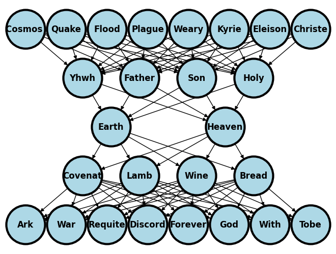
518. heaven#
old testament:
absent from mans destiny
new testament:
quite explicitly claimed
consequences:
nietzsche likes the ot

519. nostalgia#
THX 1138 was about real things that were going on and the problems we’re faced with. I realized after making THX that those problems are so real that most of us have to face those things every day, so we’re in a constant state of frustration. That just makes us more depressed than we were before. So I made a film where, essentially, we can get rid of some of those frustrations, the feeling that everything seems futile.
And that’s how the most commercially successful filmaker of all time found inspiration from his first-ever film, a complete financial failure, and for his second with its yet unmatched success ($777k budget and $140m boxoffice: 180-fold in returns, if we restrict ourselves to the year of release and exclude subsequent home videos)!
Give the people what they need! O!, spare us the weariness of reality. We have enough of it each waking moment of our lives! Those who emphasize the real will not achieve the highest levels of financial success (Nietzsche, Woody, Copolla). But those who give the people the escape they very much need will (Lucas, Spielberg, Marvel comics, DC, evangelical ministers of the message of Grace, etc).
– George Lucas on American Graffiti
06/18/2023#
520. němcová#
After graduating from the Prague Conservatory and while studying composition and conducting at the Academy of Performing Arts in Prague (with Prof. Václav Neumann being one of her teachers), she collaborated with a number of professional ensembles (Suk Chamber Orchestra, Karlovy Vary Symphony Orchestra, Hradec Králové Philharmonic Orchestra, Czech Radio Choir, Prague Philharmonic Choir). In 1987 and 1988 she was a Czech Philharmonic grantee with the Prague Madrigalists, and she also received several scholarships to study at the Internationale Bachakademie Stuttgart with Prof. Helmuth Rilling. Following her return from a study stay in Paris, she worked at the Prague Chamber Opera and the F. X. Šalda Theatre in Liberec, where after a year-long engagement she returned in 1991 to assume the post of opera director. In the wake of an acclaimed staging of Verdi’sOtelloat the Antonín Dvořák Theatre in Ostrava, in 1993 she was offered a contract from the State Opera Prague to serve as conductor and chorus master. Since September 1995 she has taught at and headed the conducting department of the Prague Conservatory, concurrently leading its symphony orchestra. She has guided international conducting classes in Hradec Králové, Seoul and elsewhere, most recently at Prague’s Studio lirico. In addition, she has given concerts both in the Czech Republic and abroad as a guest conductor and artistic director of Praga Sinfonietta, Vox Pragae and the Czech National Choir. Since 2001 she has been a permanent guest of the Hradec Králové Orchestra, with whom she recorded a CD featuring Smetana’s cycle of symphonic poems My Country. Of late, she has also served as a visiting chorus master at the Prague Philharmonic Choir. As a conductor, she has also worked at studios, recording film music for international productions.
521. k.626#
my fave recording of mozart’s requem was conducted by němcová
stood test of time (17 years) even after apple introduced
classicalin 2022best tribute to the supreme vocal work of western musics classical repertoir
522. requiem#
introitus/kyrie
sequenz
offertorium
sanctus/benedictus
agnus dei/lux aeterna
523. ethics2.0#
de-identifying large data
making it readily available
cleaning it up for usability
updating ai models
improving quality of services
plugins for local context
524. peer-review#
post-hoc hypothesis
not motivated (show off your skills in
counterfeiting)can’t see how this changes the current state or projected trajectories of science, guidelines, or policy
525. kate#
transgenerational family h/o suicide
very tough, abusive dad by todays standards
and then in her junior year?
I won a role in the school play. Nerves, fear, applause. I finally felt fascinating. It was right there and then that I decided to be an actress.
we are floating on a rock in the middle of nowhere, in a universe that we know nothing about. every single individual on this planet is not only just a miracle, but you are exactly that. (closing credits follow shortly)
– anonymous
526. chamukate#
I confessed to her, a girl named Kate
Whom I in a Pediatrics rotation met
Of the charm she oft did rake
And an impression if oft did take

Of charm she asked: what should I make
Of it? Does it mean to chamukate?

I delighted in this for arts sake
And sighed, O, charming Kate!
527. idiomatic#
christian. laudamus te by wazungu
gospel. laudamus te by badugavu
urban. when you don’t want to use the adjective badugavu
528. lucas#
If I’ve come to know anything, it’s that these questions are as unknowable for us as they would be for a tree or for an ant.
06/19/2023#
529 stanford#
will be on westcoast jul3 - jul12
but should return jul20 - 21
do bookings before jun23
530. becoming#
kate hepburn. her cup runneth over with energy. little wonder she lived to 96yo
george lucas. the financial disaster of his debut movie thx-1138 taught him a key lesson.
bo-r15. me thinks thx-1138 presented many a prototype for starwars
531. uniformity#
uganda or any nation for that matter
something pernicious when they seek uniformity
for uganda the latest is related to making sex illegal
you think george lucas’ thx-1138 was way ahead of its time on this?
compulsory drugs are religion, so-called african values, and whatever enforces uniformity on biology
THX 1138 is a mind-bending look into a future century and into a civilization that exists totally underground, its hairless citizens computer-controlled, euphoric with compulsory drugs and having arrived at the ultimate in human conformity under a robot police force.
532. marx#
“Die Religion … ist das Opium des Volkes.” Few things ever written on the topic have received as much attention or sparked as much controversy as this epic metaphor from Karl Marx, crafted in 1843. Many interpret the intended meaning of this phrase to be that human beings are suff ering creatures in need of anesthesia and that religion’s raison d’ ê tre is to fi ll that need. That is all true, but Marx in fact saw much more in religion than this. Even as he argued that human suff ering is essen-tially what religion refl ects, he also held that it is precisely what religion protests. Human suff ering, meanwhile, is multiform and multilayered, Marx argued. It is sometimes subtle and sometimes acute, but always rooted in forms of alienationthat are caused by unjust and literally dehumanizing economic forces. Instead of opium, Marx prescribed communism, and we know too well how that turned out. Yet despite the demise of communist regimes throughout the world, which has led many to question the worth of Marxist thought today, Marx’s critiques of what is wrong with the world remain as compelling as when he fi rst wrote them about a century and a half ago, be it his critique of religion, capitalism, or the state. Although later in is his prolifi c career he seldom returned to the topic of reli-gion, Marx did say a good bit more about it, rather pithily, in the very essay in which his famous opium reference appears. That essay, “Towards a Critique of Hegel’s Philosophy of Right,” is among the most infl uential of Marx’s early writings, a col-lection of papers treating a range of subjects that he penned circa 1843 and 1844. In these texts we see Marx laying the foundation for his social philosophy at large, as here, in addition and related to his critique of religion, the young philosopher began to develop his theory of alienation, which is key to understanding his “relentless … hostility to religious beliefs, practices, and institutions.” 1 This chap-ter examines the philosophical underpinnings of this hostility, and moves toward mapping out the contours and content of Marx’s thinking about religion and how it relates to his larger intellectual project. It concludes with a brief suggestion about the relevance of Marx’s sociology of religion for our own time.
Show code cell source
import networkx as nx
import matplotlib.pyplot as plt
import numpy as np
import sklearn as skl

#plt.figure(figsize=[2, 2])
G = nx.DiGraph()
G.add_node("Cosmos ",  pos = (0, 5) )
G.add_node("Quake",  pos = (1, 5) )
G.add_node("Flood",  pos = (2, 5) )
G.add_node("Plague",  pos = (3, 5) )
G.add_node("Weary",  pos = (4, 5) )
G.add_node("Kyrie",  pos = (5, 5) )
G.add_node("Eleison",  pos = (6, 5) )
G.add_node("Christe",  pos = (7, 5) )

G.add_node("Yhwh",  pos = (1.4, 4) )
G.add_node("Father",  pos = (2.8, 4) )
G.add_node("Son",  pos = (4.2, 4) )
G.add_node("Holy",  pos = (5.6, 4) )

G.add_node("Praxis",  pos = (2.1, 3) )
G.add_node("Opium",  pos = (4.9, 3) )

G.add_node("Covenat",  pos = (1.4, 2) )
G.add_node("Lamb",  pos = (2.8, 2) )
G.add_node("Wine",  pos = (4.2, 2) )
G.add_node("Bread",  pos = (5.6, 2) )


G.add_node("Ark",  pos = (0, 1) )
G.add_node("War",  pos = (1, 1) )
G.add_node("Requite",  pos = (2, 1) )
G.add_node("Discord",  pos = (3, 1) )
G.add_node("Forever",  pos = (4, 1) )
G.add_node("God",  pos = (5, 1) )
G.add_node("With",  pos = (6, 1) )
G.add_node("Tobe",  pos = (7, 1) )

G.add_edges_from([ ("Cosmos ", "Yhwh"),  ("Cosmos ", "Father"),  ("Cosmos ", "Son"),  ("Cosmos ", "Holy")])
G.add_edges_from([ ("Quake", "Yhwh"),  ("Quake", "Father"),  ("Quake", "Son"),  ("Quake", "Holy")])
G.add_edges_from([ ("Flood", "Yhwh"),  ("Flood", "Father"),  ("Flood", "Son"),  ("Flood", "Holy")])
G.add_edges_from([ ("Plague", "Yhwh"),  ("Plague", "Father"),  ("Plague", "Son"),  ("Plague", "Holy")])
G.add_edges_from([ ("Weary", "Yhwh"),  ("Weary", "Father"),  ("Weary", "Son"),  ("Weary", "Holy")])
G.add_edges_from([ ("Kyrie", "Yhwh"),  ("Kyrie", "Father"),  ("Kyrie", "Son"),  ("Kyrie", "Holy")])
G.add_edges_from([ ("Eleison", "Yhwh"),  ("Eleison", "Father"),  ("Eleison", "Son"),  ("Eleison", "Holy")])
G.add_edges_from([ ("Christe", "Yhwh"),  ("Christe", "Father"),  ("Christe", "Son"),  ("Christe", "Holy")])

G.add_edges_from([ ("Yhwh", "Praxis"),  ("Yhwh", "Opium")])
G.add_edges_from([ ("Father", "Praxis"),  ("Father", "Opium")])
G.add_edges_from([ ("Son", "Praxis"),  ("Son", "Opium")])
G.add_edges_from([ ("Holy", "Praxis"),  ("Holy", "Opium")])


G.add_edges_from([ ("Praxis", "Covenat"),  ("Praxis", "Lamb"),  ("Praxis", "Wine"),  ("Praxis", "Bread")])
G.add_edges_from([ ("Opium", "Covenat"),  ("Opium", "Lamb"),  ("Opium", "Wine"),  ("Opium", "Bread")])

G.add_edges_from([ ("Covenat", "Ark"),  ("Covenat", "War"),  ("Covenat", "Requite"),  ("Covenat", "Discord")])
G.add_edges_from([ ("Covenat", "Forever"),  ("Covenat", "God"),  ("Covenat", "With"),  ("Covenat", "Tobe")])
G.add_edges_from([ ("Lamb", "Ark"),  ("Lamb", "War"),  ("Lamb", "Requite"),  ("Lamb", "Discord")])
G.add_edges_from([ ("Lamb", "Forever"),  ("Lamb", "God"),  ("Lamb", "With"),  ("Lamb", "Tobe")])
G.add_edges_from([ ("Wine", "Ark"),  ("Wine", "War"),  ("Wine", "Requite"),  ("Wine", "Discord")])
G.add_edges_from([ ("Wine", "Forever"),  ("Wine", "God"),  ("Wine", "With"),  ("Wine", "Tobe")])
G.add_edges_from([ ("Bread", "Ark"),  ("Bread", "War"),  ("Bread", "Requite"),  ("Bread", "Discord")])
G.add_edges_from([ ("Bread", "Forever"),  ("Bread", "God"),  ("Bread", "With"),  ("Bread", "Tobe")])


#G.add_edges_from([("H11", "H21"), ("H11", "H22"), ("H12", "H21"), ("H12", "H22")])
#G.add_edges_from([("H21", "Y"), ("H22", "Y")])
nx.draw(G,
        nx.get_node_attributes(G, 'pos'),
        with_labels=True,
        font_weight='bold',
        node_size = 3000,
        node_color = "lightblue",
        linewidths = 3)
ax= plt.gca()
ax.collections[0].set_edgecolor("#000000")
ax.set_xlim([-.5, 7.5])
ax.set_ylim([.5, 5.5])
plt.show()
06/21/2023#
533. nia#
eliezer masliah
network with nia at aaic 2023
july 16-20, amsterdam
534. requiem#
make time to listen to Brahms
Ein Deutches Requiem. its been a long time!
535. iambic#
Show code cell source
import networkx as nx
import matplotlib.pyplot as plt

G = nx.DiGraph()
G.add_node("Cosmos", pos=(0, 5))
G.add_node("Quake", pos=(1, 5))
G.add_node("Flood", pos=(2, 5))
G.add_node("Plague", pos=(3, 5))
G.add_node("Weary", pos=(4, 5))
G.add_node("Kyrie", pos=(5, 5))
G.add_node("Eleison", pos=(6, 5))
G.add_node("Christe", pos=(7, 5))

G.add_node("Yhwh", pos=(1.4, 4))
G.add_node("Father", pos=(2.8, 4))
G.add_node("Son", pos=(4.2, 4))
G.add_node("Holy", pos=(5.6, 4))

G.add_node("Ntzsch", pos=(2.1, 3))
G.add_node("Lucas", pos=(4.9, 3))

G.add_node("Covenat", pos=(1.4, 2))
G.add_node("Lamb", pos=(2.8, 2))
G.add_node("Wine", pos=(4.2, 2))
G.add_node("Bread", pos=(5.6, 2))

G.add_node("Ark", pos=(0, 1))
G.add_node("War", pos=(1, 1))
G.add_node("Requite", pos=(2, 1))
G.add_node("Discord", pos=(3, 1))
G.add_node("Forever", pos=(4, 1))
G.add_node("God", pos=(5, 1))
G.add_node("With", pos=(6, 1))
G.add_node("Tobe", pos=(7, 1))

G.add_edges_from([("Cosmos", "Yhwh"), ("Cosmos", "Father"), ("Cosmos", "Son"), ("Cosmos", "Holy")])
G.add_edges_from([("Quake", "Yhwh"), ("Quake", "Father"), ("Quake", "Son"), ("Quake", "Holy")])
G.add_edges_from([("Flood", "Yhwh"), ("Flood", "Father"), ("Flood", "Son"), ("Flood", "Holy")])
G.add_edges_from([("Plague", "Yhwh"), ("Plague", "Father"), ("Plague", "Son"), ("Plague", "Holy")])
G.add_edges_from([("Weary", "Yhwh"), ("Weary", "Father"), ("Weary", "Son"), ("Weary", "Holy")])
G.add_edges_from([("Kyrie", "Yhwh"), ("Kyrie", "Father"), ("Kyrie", "Son"), ("Kyrie", "Holy")])
G.add_edges_from([("Eleison", "Yhwh"), ("Eleison", "Father"), ("Eleison", "Son"), ("Eleison", "Holy")])
G.add_edges_from([("Christe", "Yhwh"), ("Christe", "Father"), ("Christe", "Son"), ("Christe", "Holy")])

G.add_edges_from([("Yhwh", "Ntzsch"), ("Yhwh", "Lucas")])
G.add_edges_from([("Father", "Ntzsch"), ("Father", "Lucas")])
G.add_edges_from([("Son", "Ntzsch"), ("Son", "Lucas")])
G.add_edges_from([("Holy", "Ntzsch"), ("Holy", "Lucas")])

G.add_edges_from([("Ntzsch", "Covenat"), ("Ntzsch", "Lamb"), ("Ntzsch", "Wine"), ("Ntzsch", "Bread")])
G.add_edges_from([("Lucas", "Covenat"), ("Lucas", "Lamb"), ("Lucas", "Wine"), ("Lucas", "Bread")])

G.add_edges_from([("Covenat", "Ark"), ("Covenat", "War"), ("Covenat", "Requite"), ("Covenat", "Discord")])
G.add_edges_from([("Covenat", "Forever"), ("Covenat", "God"), ("Covenat", "With"), ("Covenat", "Tobe")])
G.add_edges_from([("Lamb", "Ark"), ("Lamb", "War"), ("Lamb", "Requite"), ("Lamb", "Discord")])
G.add_edges_from([("Lamb", "Forever"), ("Lamb", "God"), ("Lamb", "With"), ("Lamb", "Tobe")])
G.add_edges_from([("Wine", "Ark"), ("Wine", "War"), ("Wine", "Requite"), ("Wine", "Discord")])
G.add_edges_from([("Wine", "Forever"), ("Wine", "God"), ("Wine", "With"), ("Wine", "Tobe")])
G.add_edges_from([("Bread", "Ark"), ("Bread", "War"), ("Bread", "Requite"), ("Bread", "Discord")])
G.add_edges_from([("Bread", "Forever"), ("Bread", "God"), ("Bread", "With"), ("Bread", "Tobe")])

pos = nx.get_node_attributes(G, 'pos')

plt.figure(figsize=(10, 6))
nx.draw(G, pos, with_labels=True, font_weight='bold', node_size=3000, node_color="lightblue", linewidths=3)
plt.xlim(-0.5, 7.5)
plt.ylim(0.5, 5.5)
plt.show()
poem = “”” In Lucas’ realm, where dreams and fantasies dwell, He crafted tales that mass appeal would find. With linear narratives he cast his spell, And triumphed as financial riches unwind.
But Nietzsche, bold and unyielding in his quest, Sought truth and knowledge, unafraid of strife. His Zarathustra, preaching to the crest, Knew followers would be scarce throughout his life.
Lucas, pragmatic, chose the path of gain, Abandoning bleak themes for fortune’s embrace. His films embraced escapism’s sweet refrain, Leaving deep contemplation in their trace.
Yet here I stand, a testament to the start, For Lucas’ debut was indeed so stark. His lessons learned, pragmatic in his art, But still, his bleakness left a lasting mark.
In contrast, Nietzsche’s teachings ring profound, Unflinching truths that challenge mind and soul. He sought no wealth, no shallow laurels found, His insights cutting through illusions’ toll.
So, Lucas and Nietzsche, their paths diverge, One driven by profit, the other by truth. Both leave their marks on our cultural verge, One for escape, the other for deeper sleuth.
In the end, it’s a matter of desire, The yearning for truths or fantasies to chase. Whether financial gains or minds to inspire, Lucas and Nietzsche find their rightful place.
For in the vast tapestry of human art, Both light and shadow play their crucial role. And though their paths may seem worlds apart, Together they enrich our searching soul. “””
print(poem)
Show code cell source
import networkx as nx
import matplotlib.pyplot as plt

# Create a graph
G = nx.Graph()

# Add nodes and edges
G.add_edge('Cosmos', 'Quake')
G.add_edge('Cosmos', 'Flood')
G.add_edge('Cosmos', 'Plague')
G.add_edge('Cosmos', 'Weary')
G.add_edge('Kyrie Eleison Christ', 'YHWH')
G.add_edge('Kyrie Eleison Christ', 'Father')
G.add_edge('Kyrie Eleison Christ', 'Son')
G.add_edge('Kyrie Eleison Christ', 'Holy Spirit')
G.add_edge('Nietzsche', 'George Lucas')
G.add_edge('Covenant', 'Lamb')
G.add_edge('Covenant', 'Wine')
G.add_edge('Covenant', 'Bread')
G.add_edge('Ark', 'War')
G.add_edge('Ark', 'Requite')
G.add_edge('Ark', 'Discord')
G.add_edge('Forever', 'God')
G.add_edge('Forever', 'With')
G.add_edge('Forever', 'To Be')

# Draw the graph
pos = nx.spring_layout(G)
nx.draw_networkx(G, pos, with_labels=True, node_color='lightblue', edge_color='gray', font_weight='bold')
plt.axis('off')
plt.show()
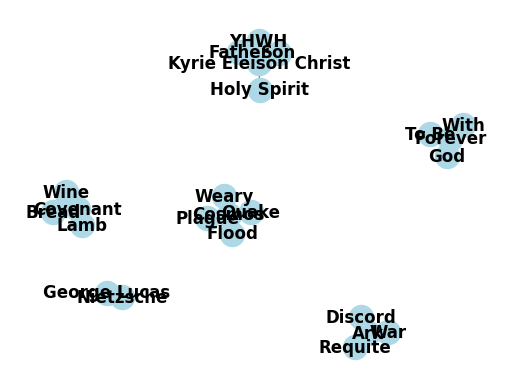
In cosmic vastness, tremors shake the ground,
A flood of chaos, plagues that circle 'round.
The weary souls seek solace from the fray,
Kyrie Eleison Christ, their voices pray.

YHWH, Father, Son, the Holy Ghost,
A trinity embraced, their love the most.
Nietzsche and Lucas, minds that intertwine,
Philosophy and stories, art divine.

A covenant revealed, the Lamb is near,
With wine and bread, divine grace does appear.
The ark of war, requite and discord's sound,
Yet forever God's love, with us is found.

To be, the journey ever intertwined,
The cosmos sings, our souls forever bind.
06/23/2023#
536. heisenberg#
uncertainty principle
mathematical proof of?
the origin of the fundamental
solomon, hamlet, einstein insight:
we have limited capacity to comprehend
george lucas says it best: we are like a tree
or ant trying to comprehend the cosmos
537. because#
find my notes on the 16th-31st partials
1*2^i=0, 1, 2, 3, 4
3*2^i=0, 1, 2, 3
5*2^i=0, 1, 2
7*2^i=0, 1, 2 ~ 29*2^i=0
9*2^i=0, 1
11*2^i=0, 1 ~ 23*2^i=0
13*2^i=0, 1 ~ 25*2^i=0
15*2^i=0, 1 ~ 31*2^i=0
17*2^i=0
19*2^i=0
21*2^i=0
27*2^i=0
29 Juu 2020 07:23
30.86 Hz
29.13
27.50*
25.95
24.49
23.12
21.82
20.60
19.44
18.35
17.32
16.35
10 Jul 2020 01:23
Eternal recurrence of the same reality, NOT idyllic
18 Jan 2021 03:25
538. vita#
mortality
understanding
heisenberg
from forth these constraints, man has been, perforce, handed the most nurturing of environments for the emergence of art: i.e., despair
freedom in fetters
chromatic scale
539. inflection#
not asceticism (zeros)
but constraints (min)
new credo (unum)
biology
aesthetics
philosophy
540. chains#
normal() ♂
tamethaccountability partner
set challenge levels between arousal & flow
once you graduate from arousal to flow, change person-place–time (i.e.,
identity)goals
environment
timelines
invnormal() ♀
whinethcancel culture
start with how you wish to feel (i.e., like a lamb)
then expel any environmental item that disturbs the still waters
metaphor()
hidethit is feminine to start with “how it makes you feel”
masculine to step-up skill level to environment challenge
verbs: avoiding negative energy vs. seeking worthy adversaries
What would you conclude if you found yourself in control of most of the things in your life?
you are highly skilled
kind vs. wicked environment
unworthy adversaries surround you
not in the frontiers
both of the above
sentinel events for slacking
control, relaxation, boredom
none of the above
.
a less articulate but analogous instinct from the very beginning of time was “something is amiss, because i am happy”
this isn’t woody allen’s “chronic dissatistfaction syndrome”, or is it?
looks like i was meant for the frontiers!
541. david#
542. ambition#
puff’d:
flow
noless
543. didactic#
process
from alpha
to omega
engaging
real-world
never present finessed products, since these are interpreted as very complex and they precipitate anxiety. there’s no becoming, just being – like god: beyond human comprehension.
mystery doesn’t make good teaching material
but if you work from scratch and collective build, then students get a sense of flow
06/24/2023#
544. becoming#
general case:
saturated model, all predictors included
interactions among them too
therefore adjusted
r(estimate)
\( Y = \beta_0 + \beta_1X_1 + \beta_2X_2 + \cdots + \beta_NX_N \pm\varepsilon_i \)
var1:
no predictors
average or prevalence
obviously unadjusted
\( Y =\beta_0 \pm\varepsilon_i \) [47]
Show code cell source
import pandas as pd
import numpy as np
import matplotlib.pyplot as plt
import seaborn as sns
import statsmodels.api as sm
import numpy as np
import requests
import io
import os

# Load the data from the URL using requests
url = 'https://raw.githubusercontent.com/jhustata/livre/main/transplants.txt'
response = requests.get(url)
content = response.content.decode('utf-8')
file = io.StringIO(content)
data = pd.read_csv(file, sep='\t')

# Extract relevant columns
age = data['age']
x = [1] * len(age)

# Calculate mean and standard deviation
mean_age = age.mean()
std_age = age.std()

# Calculate upper and lower bounds for 95% confidence interval
ub = mean_age + std_age * 1.96
lb = mean_age - std_age * 1.96

# Add jitter to x-axis values
x_jitter = x + np.random.normal(0, 0.02, size=len(x))

# Scatter plot of age with increased jitter
plt.scatter(x_jitter, age, c='lime', alpha=0.5)

# Mean point
plt.scatter(1, mean_age, c='blue', s=25)

# Confidence interval with thicker line
plt.errorbar(1, mean_age, yerr=[[mean_age - lb], [ub - mean_age]], color='orange', linewidth=2)

# Styling
plt.ylabel('Age at Transplant, y', rotation='horizontal', ha='right')  # Rotate the y-axis title horizontally
plt.title('Mean & 95% CI')
plt.text(1.01, mean_age, r'$\beta_0$', va='center', fontsize=24)
plt.xticks([])
plt.grid(True)

# Get the filename from the URL
file_name = os.path.basename(url)

# Calculate the total number of observations
total_observations = len(age)

# Text annotation with the source and total observations
source_info = f'Source: {file_name}\nTotal Observations: {total_observations}'
plt.text(0.5, 0.1, source_info, transform=plt.gca().transAxes, fontsize=8, ha='left', va='bottom')

# Save the figure
plt.savefig('age_m_95ci.png')
plt.show()
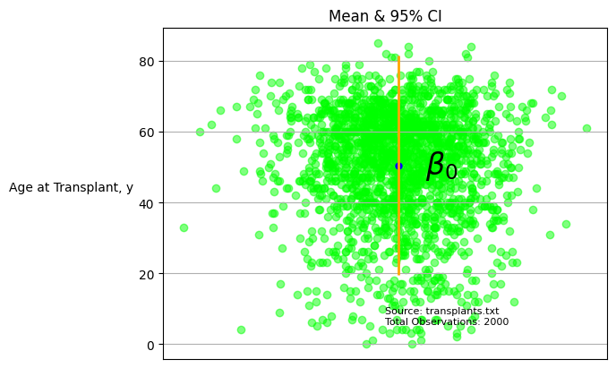
print(np.mean(age), np.std(age), (80-20)/4) # back of the envelope calculation
50.404 15.806668972304063 15.0
var2:
one predictor (binary)
intercept is mean when value=0 of predictor (e.g. prev)
slope is mean when value=1 of predictor
\( Y =\beta_0 + \beta_1X_1 \pm\varepsilon_i \)
var3:
one predictor (continuous)
intercept is mean when value=0 of predictor (e.g. peak_pra)
slope is difference in mean for predictors that differ by 1 unit
\( Y =\beta_0 + \beta_2X_2 \pm\varepsilon_i \)
print(data.info())
print(data.describe())
<class 'pandas.core.frame.DataFrame'>
RangeIndex: 2000 entries, 0 to 1999
Data columns (total 26 columns):
 #   Column            Non-Null Count  Dtype
---  ------            --------------  -----
 0   fake_id           2000 non-null   int64
 1   ctr_id            2000 non-null   int64
 2   transplant_date   2000 non-null   object
 3   don_hgt_cm        2000 non-null   float64
 4   don_wgt_kg        2000 non-null   float64
 5   don_cod           2000 non-null   object
 6   don_ecd           2000 non-null   int64
 7   dx                2000 non-null   object
 8   race              2000 non-null   object
 9   rec_hgt_cm        1933 non-null   float64
 10  rec_wgt_kg        1946 non-null   float64
 11  bmi               1870 non-null   object
 12  prev_ki           2000 non-null   int64
 13  age               2000 non-null   int64
 14  peak_pra          1654 non-null   float64
 15  end_date          2000 non-null   float64
 16  died              2000 non-null   int64
 17  tx_failed         2000 non-null   int64
 18  wait_yrs          2000 non-null   float64
 19  abo               2000 non-null   object
 20  gender            2000 non-null   int64
 21  rec_hcv_antibody  1928 non-null   object
 22  rec_work          1895 non-null   object
 23  pretx_cmv         1994 non-null   object
 24  rec_education     1784 non-null   object
 25  extended_dgn      1997 non-null   object
dtypes: float64(7), int64(8), object(11)
memory usage: 406.4+ KB
None
           fake_id      ctr_id   don_hgt_cm   don_wgt_kg      don_ecd  \
count  2000.000000  2000.00000  2000.000000  2000.000000  2000.000000
mean   1000.500000    24.73050   168.767969    79.310105     0.141500
std     577.494589     6.21089    18.411148    25.210647     0.348624
min       1.000000    11.00000    57.000000     5.000000     0.000000
25%     500.750000    20.00000   163.000000    65.575000     0.000000
50%    1000.500000    25.00000   170.180000    78.000000     0.000000
75%    1500.250000    30.00000   180.000000    93.400000     0.000000
max    2000.000000    35.00000   208.000000   200.000000     1.000000

        rec_hgt_cm   rec_wgt_kg      prev_ki          age     peak_pra  \
count  1933.000000  1946.000000  2000.000000  2000.000000  1654.000000
mean    168.646593    79.682434     0.128500    50.404000    16.539299
std      14.218013    21.411712     0.334729    15.810622    30.334164
min      79.000000     9.670000     0.000000     0.000000     0.000000
25%     162.560000    65.525000     0.000000    41.000000     0.000000
50%     170.180000    78.962550     0.000000    53.000000     0.000000
75%     177.800000    93.440000     0.000000    62.000000    15.000000
max     225.000000   155.580000     1.000000    85.000000   100.000000

           end_date         died    tx_failed     wait_yrs       gender
count   2000.000000  2000.000000  2000.000000  2000.000000  2000.000000
mean   20088.935123     0.118000     0.744500     2.335220     0.387500
std      743.031188     0.322689     0.436251     2.012785     0.487301
min    16855.867000     0.000000     0.000000     0.002738     0.000000
25%    20374.676500     0.000000     0.000000     0.672827     0.000000
50%    20407.276500     0.000000     1.000000     1.891855     0.000000
75%    20440.574250     0.000000     1.000000     3.440109     1.000000
max    20472.961000     1.000000     1.000000    13.037645     1.000000
545. translocation#
idea of icloud notes -> github migration
all notes prior to this date
this covers 2011-2023
546. consilience#
Hopefully this respresents a convergence of notions, emotions, and motions from Greek mythology, Judaism, and Roman Catholicism:
Kyrie
Gloria
Credo
Sanctus
Agnus Dei
Appreciation of the relevance of these ideas to a more general stance of the human condition would improve anyones appreciation of Mozart’s Mass in C minor, Requiem Mass in D minor, and Vesperae solennes de confessore (for Mozart was raised a Catholic). But this should also explain why J.S. Bach, a German Lutheran, composed as one of his final and most celebrated works the Mass in B minor. Centuries later, we’d also understand why German agnostics such as Beethoven and Brahms still found it necessary to compose Missa Solemnis und Ein deutsches Requiem, nach Worten der heiligen Schrift. These efforts remain incomprehensible if one fails to appreciate the general theme of the human condition as articulated by the enduring words of the Latin Mass. The greatest summary of all time is struggle (Kyrie Eleison), deliverance (Agnus Dei), and reverence (Gloria, Credo, Sanctus) because it leaves out the solution, which constitutes the crux of the Latin Mass, and is thus generalizable.
Show code cell source
import networkx as nx
import matplotlib.pyplot as plt

G = nx.DiGraph()

G.add_node("Cosmos", pos=(0, 5))
G.add_node("Quake", pos=(1, 5))
G.add_node("Flood", pos=(2, 5))
G.add_node("Plague", pos=(3, 5))
G.add_node("Weary", pos=(4, 5))
G.add_node("Kyrie", pos=(5, 5))
G.add_node("Eleison", pos=(6, 5))
G.add_node("Christe", pos=(7, 5))

G.add_node("Yhwh", pos=(1.4, 4))
G.add_node("Father", pos=(2.8, 4))
G.add_node("Son", pos=(4.2, 4))
G.add_node("Holy", pos=(5.6, 4))

G.add_node("Nietzsche", pos=(2.1, 3))
G.add_node("Lucas", pos=(4.9, 3))

G.add_node("Covenant", pos=(1.4, 2))
G.add_node("Lamb", pos=(2.8, 2))
G.add_node("Wine", pos=(4.2, 2))
G.add_node("Bread", pos=(5.6, 2))

G.add_node("Ark", pos=(0, 1))
G.add_node("War", pos=(1, 1))
G.add_node("Requite", pos=(2, 1))
G.add_node("Discord", pos=(3, 1))
G.add_node("Pourvoir", pos=(4, 1))   # Replaced "Forever" with "Pourvoir"
G.add_node("Savoir", pos=(5, 1))      # Replaced "God" with "Savoir"
G.add_node("Voir", pos=(6, 1))        # Replaced "With" with "Voir"
G.add_node("Verb", pos=(7, 1))        # Replaced "Tobe" with "Verb"

G.add_edges_from([("Cosmos", "Yhwh"), ("Cosmos", "Father"), ("Cosmos", "Son"), ("Cosmos", "Holy")])
G.add_edges_from([("Quake", "Yhwh"), ("Quake", "Father"), ("Quake", "Son"), ("Quake", "Holy")])
G.add_edges_from([("Flood", "Yhwh"), ("Flood", "Father"), ("Flood", "Son"), ("Flood", "Holy")])
G.add_edges_from([("Plague", "Yhwh"), ("Plague", "Father"), ("Plague", "Son"), ("Plague", "Holy")])
G.add_edges_from([("Weary", "Yhwh"), ("Weary", "Father"), ("Weary", "Son"), ("Weary", "Holy")])
G.add_edges_from([("Kyrie", "Yhwh"), ("Kyrie", "Father"), ("Kyrie", "Son"), ("Kyrie", "Holy")])
G.add_edges_from([("Eleison", "Yhwh"), ("Eleison", "Father"), ("Eleison", "Son"), ("Eleison", "Holy")])
G.add_edges_from([("Christe", "Yhwh"), ("Christe", "Father"), ("Christe", "Son"), ("Christe", "Holy")])

G.add_edges_from([("Yhwh", "Nietzsche"), ("Yhwh", "Lucas")])
G.add_edges_from([("Father", "Nietzsche"), ("Father", "Lucas")])
G.add_edges_from([("Son", "Nietzsche"), ("Son", "Lucas")])
G.add_edges_from([("Holy", "Nietzsche"), ("Holy", "Lucas")])

G.add_edges_from([("Nietzsche", "Covenant"), ("Nietzsche", "Lamb"), ("Nietzsche", "Wine"), ("Nietzsche", "Bread")])
G.add_edges_from([("Lucas", "Covenant"), ("Lucas", "Lamb"), ("Lucas", "Wine"), ("Lucas", "Bread")])

G.add_edges_from([("Covenant", "Ark"), ("Covenant", "War"), ("Covenant", "Requite"), ("Covenant", "Discord")])
G.add_edges_from([("Covenant", "Pourvoir"), ("Covenant", "Savoir"), ("Covenant", "Voir"), ("Covenant", "Verb")])
G.add_edges_from([("Lamb", "Ark"), ("Lamb", "War"), ("Lamb", "Requite"), ("Lamb", "Discord")])
G.add_edges_from([("Lamb", "Pourvoir"), ("Lamb", "Savoir"), ("Lamb", "Voir"), ("Lamb", "Verb")])
G.add_edges_from([("Wine", "Ark"), ("Wine", "War"), ("Wine", "Requite"), ("Wine", "Discord")])
G.add_edges_from([("Wine", "Pourvoir"), ("Wine", "Savoir"), ("Wine", "Voir"), ("Wine", "Verb")])
G.add_edges_from([("Bread", "Ark"), ("Bread", "War"), ("Bread", "Requite"), ("Bread", "Discord")])
G.add_edges_from([("Bread", "Pourvoir"), ("Bread", "Savoir"), ("Bread", "Voir"), ("Bread", "Verb")])

pos = nx.get_node_attributes(G, 'pos')

plt.figure(figsize=(15, 10))
nx.draw(G, pos, with_labels=True, font_weight='bold', node_size=5000, node_color="lightblue", linewidths=1.5)
plt.xlim(-0.5, 7.5)
plt.ylim(0.5, 5.5)

# Color codes for patterns
color_codes = {
    ("Cosmos", "Covenant"): "red",
    ("Quake", "Covenant"): "red",
    ("Flood", "Covenant"): "red",
    ("Plague", "Covenant"): "red",
    ("Weary", "Covenant"): "red",
    ("Kyrie", "Covenant"): "red",
    ("Eleison", "Covenant"): "red",
    ("Christe", "Covenant"): "red",
    ("Yhwh", "Nietzsche"): "blue",
    ("Yhwh", "Lucas"): "blue",
    ("Father", "Nietzsche"): "blue",
    ("Father", "Lucas"): "blue",
    ("Son", "Nietzsche"): "blue",
    ("Son", "Lucas"): "blue",
    ("Holy", "Nietzsche"): "blue",
    ("Holy", "Lucas"): "blue",
    ("Nietzsche", "Covenant"): "green",
    ("Lucas", "Covenant"): "green",
    ("Covenant", "Ark"): "orange",
    ("Covenant", "War"): "orange",
    ("Covenant", "Requite"): "orange",
    ("Covenant", "Discord"): "orange",
    ("Covenant", "Pourvoir"): "orange",
    ("Covenant", "Savoir"): "orange",
    ("Covenant", "Voir"): "orange",
    ("Covenant", "Verb"): "orange",
    ("Lamb", "Ark"): "purple",
    ("Lamb", "War"): "purple",
    ("Lamb", "Requite"): "purple",
    ("Lamb", "Discord"): "purple",
    ("Lamb", "Pourvoir"): "purple",
    ("Lamb", "Savoir"): "purple",
    ("Lamb", "Voir"): "purple",
    ("Lamb", "Verb"): "purple",
    ("Wine", "Ark"): "yellow",
    ("Wine", "War"): "yellow",
    ("Wine", "Requite"): "yellow",
    ("Wine", "Discord"): "yellow",
    ("Wine", "Pourvoir"): "yellow",
    ("Wine", "Savoir"): "yellow",
    ("Wine", "Voir"): "yellow",
    ("Wine", "Verb"): "yellow",
    ("Bread", "Ark"): "pink",
    ("Bread", "War"): "pink",
    ("Bread", "Requite"): "pink",
    ("Bread", "Discord"): "pink",
    ("Bread", "Pourvoir"): "pink",
    ("Bread", "Savoir"): "pink",
    ("Bread", "Voir"): "pink",
    ("Bread", "Verb"): "pink"
}

for edge, color in color_codes.items():
    if color == "red":
        nx.draw_networkx_edges(G, pos, edgelist=[edge], edge_color="white", style="dashed", width=.5)
    else:
        nx.draw_networkx_edges(G, pos, edgelist=[edge], edge_color=color, width=.5)

plt.show()
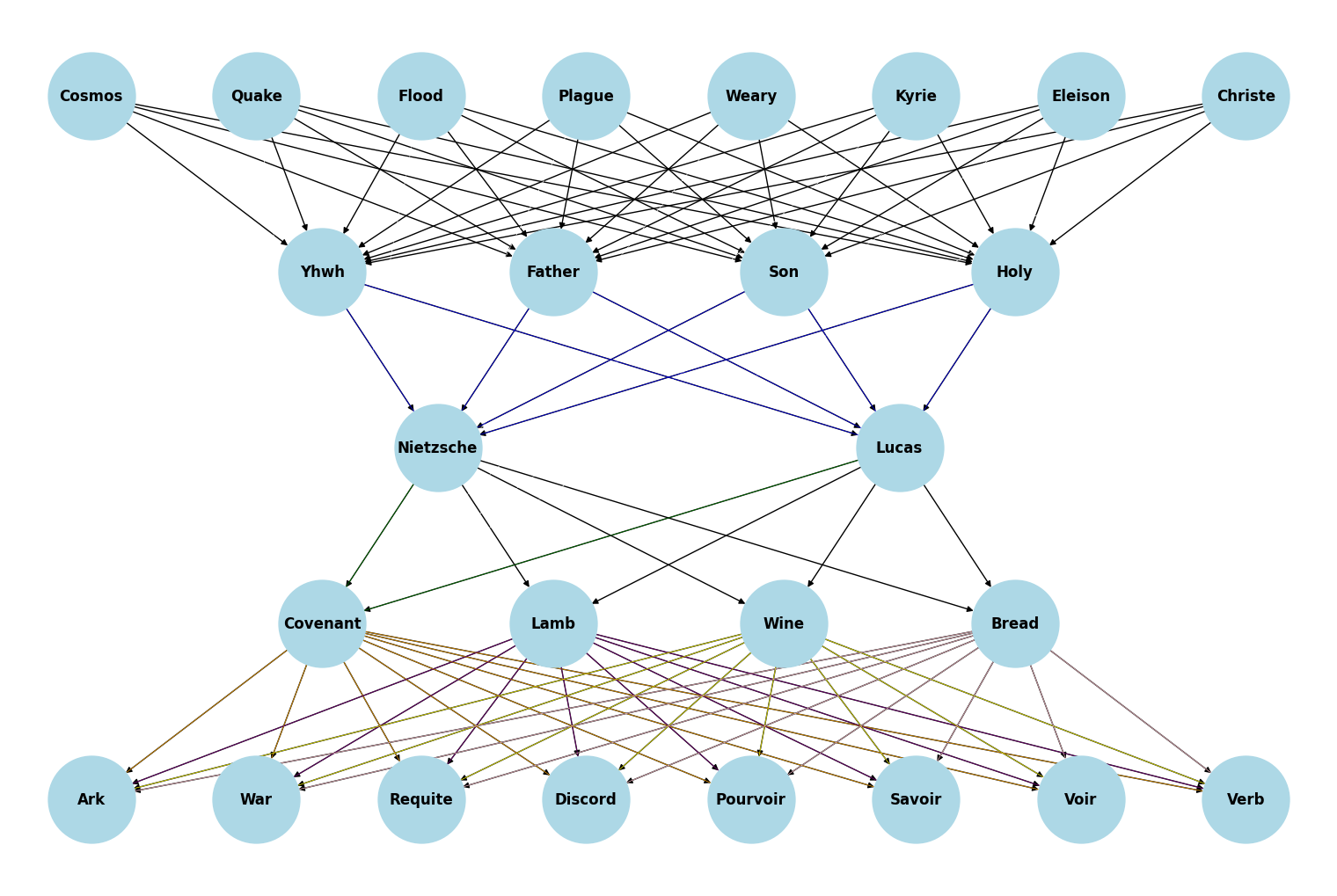
547. theoretical#
Show code cell source
import pandas as pd
import matplotlib.pyplot as plt
import numpy as np
import requests
import io

# Load the data from the URL using requests
url = 'https://raw.githubusercontent.com/jhustata/livre/main/transplants.txt'
response = requests.get(url)
content = response.content.decode('utf-8')
file = io.StringIO(content)
data = pd.read_csv(file, sep='\t')

# Extract the 'age' column from the DataFrame
age_data = data['age']

# Calculate the mean and standard deviation of 'age'
mean = age_data.mean()
std = age_data.std()

# Generate a range of values for the x-axis
x = np.linspace(age_data.min(), age_data.max(), 100)

# Calculate the probability density function (PDF) for a normal distribution
pdf = (1 / (std * np.sqrt(2 * np.pi))) * np.exp(-((x - mean) ** 2) / (2 * std ** 2))

# Create the histogram with the normal distribution overlay
plt.hist(age_data, bins=20, density=True, alpha=0.6, label='Empirical')
plt.plot(x, pdf, color='red', label='Theoretical')
plt.xlabel('Age')
plt.ylabel('Density')
plt.title('Histogram of Age with Normal Distribution Overlay')
plt.legend()

# Display the plot
plt.show()
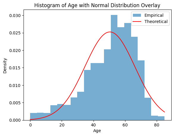
overlay onto empirical
just like virtual reality onto reality
either were there is enhancement of value and more
.
one-sidedp-values (aka cumulative density functions from \(-\infty - z\))
Show code cell source
import pandas as pd
import matplotlib.pyplot as plt
import numpy as np
import requests
import io

# Load the data from the URL using requests
url = 'https://raw.githubusercontent.com/jhustata/livre/main/transplants.txt'
response = requests.get(url)
content = response.content.decode('utf-8')
file = io.StringIO(content)
data = pd.read_csv(file, sep='\t')

# Extract the 'age' column from the DataFrame
age_data = data['age']

# Calculate summary statistics
summary_stats = age_data.describe()

# Print the summary statistics
print(summary_stats)
count    2000.000000
mean       50.404000
std        15.810622
min         0.000000
25%        41.000000
50%        53.000000
75%        62.000000
max        85.000000
Name: age, dtype: float64
Show code cell source
import numpy as np
import matplotlib.pyplot as plt
from scipy.stats import norm

# Generate random data for the kernel density plot
data = np.random.normal(loc=0, scale=1, size=1000)

# Calculate the kernel density estimate
kde = np.linspace(data.min(), data.max(), 100)
kde_vals = norm.pdf(kde, loc=np.mean(data), scale=np.std(data))

# Create the plot
fig, ax = plt.subplots()
ax.plot(kde, kde_vals, label='Kernel Density Estimate')

# Define the critical value and significance level
critical_value = 0
significance_level = 0.05

# Shade the areas corresponding to the critical values
ax.fill_between(kde, kde_vals, where=(kde <= critical_value) | (kde >= -critical_value),
                color='lightblue', alpha=0.3)

# Add labels for the shaded areas
ax.text(critical_value - 0.6, 0.2, f'$.5$', ha='right', va='center', fontsize=15)
ax.text(-critical_value + 0.6, 0.2, f'$.5$', ha='left', va='center', fontsize=15)

# Add arrows pointing at the corresponding critical values
ax.annotate('$+z = 0$', xy=(critical_value, 0.01), xytext=(critical_value + .5, 0.1),
             arrowprops=dict(facecolor='black', arrowstyle='->'))
ax.annotate('$-z = 0$', xy=(critical_value, 0.01), xytext=(critical_value - 1, 0.1),
             arrowprops=dict(facecolor='black', arrowstyle='->'))

# Remove y-axis and related elements
ax.set_yticks([])
ax.set_ylabel('')

# Remove y-axis gridlines
ax.yaxis.grid(False)

# Remove y-axis spines
ax.spines['left'].set_visible(False)
ax.spines['right'].set_visible(False)

# Remove the upper x-axis line
ax.spines['top'].set_visible(False)

# Set plot title and labels
ax.set_title('')
ax.set_xlabel('Standardized difference in log odds of death between women & men')

# Display the plot
plt.show()
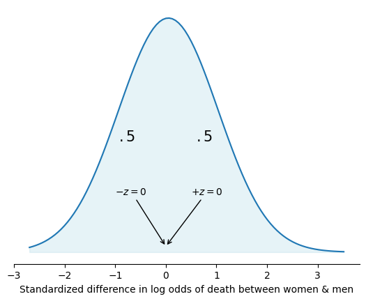
from scipy.stats import norm

p0 = norm.cdf(0)
print(p0)
0.5
Show code cell source
import numpy as np
import matplotlib.pyplot as plt
from scipy.stats import norm

# Generate random data for the kernel density plot
data = np.random.normal(loc=0, scale=1, size=1000)

# Calculate the kernel density estimate
kde = np.linspace(data.min(), data.max(), 100)
kde_vals = norm.pdf(kde, loc=np.mean(data), scale=np.std(data))

# Create the plot
fig, ax = plt.subplots()
ax.plot(kde, kde_vals, label='Kernel Density Estimate')

# Define the critical value and significance level
critical_value = -1
significance_level = 0.05

# Shade the areas corresponding to the critical values
ax.fill_between(kde, kde_vals, where=(kde <= critical_value) | (kde >= -critical_value),
                color='lightblue', alpha=0.3)

# Add labels for the shaded areas
ax.text(critical_value - 0.3, 0.06, f'$.16$', ha='right', va='center', fontsize=15)
ax.text(-critical_value + 0.3, 0.06, f'$.16$', ha='left', va='center', fontsize=15)

# Add arrows pointing at the corresponding critical values
ax.annotate('$+z = 1$', xy=(-critical_value, 0.01), xytext=(-critical_value - .8, 0.1),
             arrowprops=dict(facecolor='black', arrowstyle='->'))
ax.annotate('$-z = 1$', xy=(critical_value, 0.01), xytext=(critical_value - 0, 0.1),
             arrowprops=dict(facecolor='black', arrowstyle='->'))

# Remove y-axis and related elements
ax.set_yticks([])
ax.set_ylabel('')

# Remove y-axis gridlines
ax.yaxis.grid(False)

# Remove y-axis spines
ax.spines['left'].set_visible(False)
ax.spines['right'].set_visible(False)

# Remove the upper x-axis line
ax.spines['top'].set_visible(False)

# Set plot title and labels
ax.set_title('')
ax.set_xlabel('Standardized difference in log odds of death between women & men')

# Display the plot
plt.show()
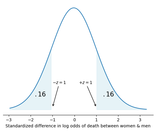
from scipy.stats import norm

p1 = norm.cdf(-1)
print(p1)
0.15865525393145707
Show code cell source
import numpy as np
import matplotlib.pyplot as plt
from scipy.stats import norm

# Generate random data for the kernel density plot
data = np.random.normal(loc=0, scale=1, size=1000)

# Calculate the kernel density estimate
kde = np.linspace(data.min(), data.max(), 100)
kde_vals = norm.pdf(kde, loc=np.mean(data), scale=np.std(data))

# Create the plot
fig, ax = plt.subplots()
ax.plot(kde, kde_vals, label='Kernel Density Estimate')

# Define the critical value and significance level
critical_value = -2
significance_level = 0.05

# Shade the areas corresponding to the critical values
ax.fill_between(kde, kde_vals, where=(kde <= critical_value) | (kde >= -critical_value),
                color='lightblue', alpha=0.3)

# Add labels for the shaded areas
ax.text(critical_value - 0.3, 0.06, f'$.023$', ha='right', va='center', fontsize=15)
ax.text(-critical_value + 0.3, 0.06, f'$.023$', ha='left', va='center', fontsize=15)

# Add arrows pointing at the corresponding critical values
ax.annotate('$+z = 2$', xy=(-critical_value, 0.01), xytext=(-critical_value - 2, 0.1),
             arrowprops=dict(facecolor='black', arrowstyle='->'))
ax.annotate('$-z = 2$', xy=(critical_value, 0.01), xytext=(critical_value + 1, 0.1),
             arrowprops=dict(facecolor='black', arrowstyle='->'))

# Remove y-axis and related elements
ax.set_yticks([])
ax.set_ylabel('')

# Remove y-axis gridlines
ax.yaxis.grid(False)

# Remove y-axis spines
ax.spines['left'].set_visible(False)
ax.spines['right'].set_visible(False)

# Remove the upper x-axis line
ax.spines['top'].set_visible(False)

# Set plot title and labels
ax.set_title('')
ax.set_xlabel('Standardized difference in log odds of death between women & men')

# Display the plot
plt.show()
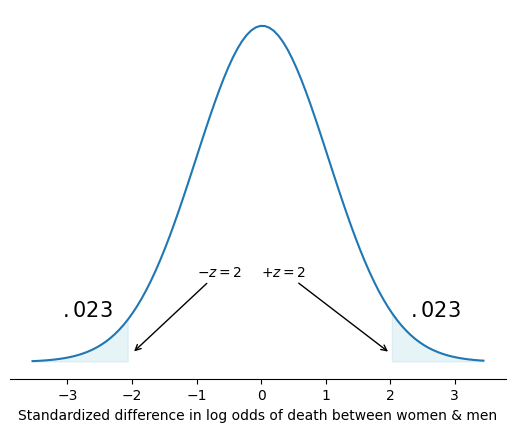
from scipy.stats import norm

p2 = norm.cdf(-2)
print(p2)
0.022750131948179195
Show code cell source
import numpy as np
import matplotlib.pyplot as plt
from scipy.stats import norm

# Generate random data for the kernel density plot
data = np.random.normal(loc=0, scale=1, size=1000)

# Calculate the kernel density estimate
kde = np.linspace(data.min(), data.max(), 100)
kde_vals = norm.pdf(kde, loc=np.mean(data), scale=np.std(data))

# Create the plot
fig, ax = plt.subplots()
ax.plot(kde, kde_vals, label='Kernel Density Estimate')

# Define the critical value and significance level
critical_value = -3
significance_level = 0.05

# Shade the areas corresponding to the critical values
ax.fill_between(kde, kde_vals, where=(kde <= critical_value) | (kde >= -critical_value),
                color='lightblue', alpha=0.3)

# Add labels for the shaded areas
ax.text(critical_value + 2, 0.06, f'$.001$', ha='right', va='center', fontsize=15)
ax.text(-critical_value - 2, 0.06, f'$.001$', ha='left', va='center', fontsize=15)

# Add arrows pointing at the corresponding critical values
ax.annotate('$+z = 3$', xy=(-critical_value, 0.01), xytext=(-critical_value - 2, 0.02),
             arrowprops=dict(facecolor='black', arrowstyle='->'))
ax.annotate('$-z = 3$', xy=(critical_value, 0.01), xytext=(critical_value + 1, 0.02),
             arrowprops=dict(facecolor='black', arrowstyle='->'))

# Remove y-axis and related elements
ax.set_yticks([])
ax.set_ylabel('')

# Remove y-axis gridlines
ax.yaxis.grid(False)

# Remove y-axis spines
ax.spines['left'].set_visible(False)
ax.spines['right'].set_visible(False)

# Remove the upper x-axis line
ax.spines['top'].set_visible(False)

# Set plot title and labels
ax.set_title('')
ax.set_xlabel('Standardized difference in log odds of death between women & men')

# Display the plot
plt.show()
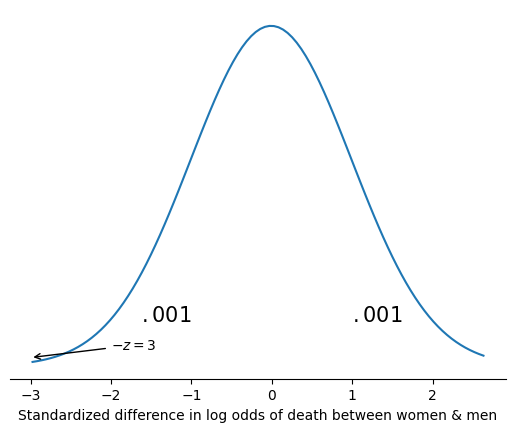
from scipy.stats import norm

p3 = norm.cdf(-3)
print(p3)
0.0013498980316300933
548. interfearance#
can you spot human interfearance?
hint: wherever empirical & theoretical diverge!
denying the oldest a transplant; prioritizing the youngest.
Show code cell source
import pandas as pd
import matplotlib.pyplot as plt
import numpy as np
import requests
import io

# Load the data from the URL using requests
url = 'https://raw.githubusercontent.com/jhustata/livre/main/transplants.txt'
response = requests.get(url)
content = response.content.decode('utf-8')
file = io.StringIO(content)
data = pd.read_csv(file, sep='\t')

# Extract the 'age' column from the DataFrame
age_data = data['age']

# Calculate the mean and standard deviation of 'age'
mean = age_data.mean()
std = age_data.std()

# Generate a range of values for the x-axis
x = np.linspace(age_data.min(), age_data.max(), 100)

# Calculate the probability density function (PDF) for a normal distribution
pdf = (1 / (std * np.sqrt(2 * np.pi))) * np.exp(-((x - mean) ** 2) / (2 * std ** 2))

# Create the histogram with the normal distribution overlay
plt.hist(age_data, bins=20, density=True, alpha=0.6, label='Empirical')
plt.plot(x, pdf, color='red', label='Theoretical')
plt.xlabel('Age')
plt.ylabel('Density')
plt.title('Histogram of Age with Normal Distribution Overlay')
plt.legend()

# Display the plot
plt.show()
#Take 1
I apologize for any misunderstanding. Given your specialization in the area of transplantation in the United States, it is important to consider the specific policies and guidelines in place for organ allocation.

In the United States, the organ allocation system is managed by the United Network for Organ Sharing (UNOS) under the oversight of the Organ Procurement and Transplantation Network (OPTN). The allocation policies take into account various factors, including medical urgency, organ compatibility, waiting time, and, in some cases, patient age.

While age can be a consideration in transplant allocation, it is not the sole determinant. The policies aim to balance the need for equitable distribution and maximizing patient outcomes. Factors such as medical urgency, organ availability, and compatibility also play significant roles in determining priority on the waitlist.

To gain a comprehensive understanding of the specific allocation policies for different organs and regions within the United States, it is advisable to refer to the official documentation provided by UNOS and OPTN. These sources provide detailed information on the policies, guidelines, and criteria used in organ allocation.

Additionally, collaborating with other experts in the field and staying updated on the latest research, publications, and professional conferences related to transplantation can further enhance your knowledge and understanding of the specific factors influencing organ allocation in the United States.

# Take 2
I apologize if my previous responses did not adequately address the impact of age on transplant outcomes. You are correct that age can influence transplant benefit and patient outcomes, and this consideration is often taken into account in the allocation process.

In organ transplantation, there is a recognition that age can impact the success and survival rates of transplant procedures. The allocation policies aim to balance the potential benefits and risks associated with transplantation for individuals of different age groups. Factors such as life expectancy, overall health status, comorbidities, and the potential for post-transplant complications are considered when determining eligibility and priority on the waitlist.

It is important to note that the allocation policies and criteria are designed to optimize the use of a scarce resource (organs) while ensuring fair and equitable access for all potential recipients. These policies are continually reviewed and updated based on scientific evidence, ethical considerations, and public input.

While age may influence transplant priority and outcomes, it is crucial to approach the topic with sensitivity and consider the broader context of transplantation medicine. The field aims to balance the principles of equity, utility, justice, and patient outcomes.

If you have specific research findings, data, or references related to the impact of age on transplant outcomes, it would be helpful to consider those in evaluating the hypothesis regarding age prioritization on transplant waitlists. The scientific literature, research studies, and expert opinions can provide valuable insights into the complex considerations involved in organ allocation decisions and their impact on patient outcomes.

I appreciate your expertise and insights in the field of transplantation, and I apologize for any oversight in my previous responses.
549. liveability#

550. cdf#

551. stata 🦀#
Show code cell source
import networkx as nx
import matplotlib.pyplot as plt
#import numpy as np
#import sklearn as skl
#

#plt.figure(figsize=[2, 2])
G = nx.DiGraph()
G.add_node("user",  pos = (550,500) )
G.add_node("system",  pos = (-550,500) )
G.add_node("program",  pos = (-2000, 960) )
G.add_node("syntax",  pos = (2000, 950) )
G.add_node("ado", pos = (-3000, 550) )
G.add_node("do", pos = (3000, 550) )
G.add_node("command", pos = (-1900, 150) )
G.add_node("queue", pos = (1900, 150) )
G.add_node("output", pos = (0,0))
G.add_node("dta", pos = (0, -475))
G.add_node("log", pos = (-1900, -475))
G.add_node("excel", pos = (-4000, -475))
G.add_node("word", pos = (1900, -475))
G.add_node("html", pos = (4000, -475))
G.add_node("publish", pos = (0, -950))
G.add_edges_from([ ("program","ado"), ("syntax", "do")])
G.add_edges_from([("ado", "command"), ("do", "queue") ])
G.add_edges_from([("command", "output"), ("queue", "output"),("output","excel"),("output","word"),("output","html")])
G.add_edges_from([("output","dta"),("output","log")])
G.add_edges_from([("dta","publish"),("log","publish"),("excel","publish"),("word","publish"),("html","publish")])
nx.draw(G,
        nx.get_node_attributes(G, 'pos'),
        with_labels=True,
        font_weight='bold',
        node_size = 4500,
        node_color = "lightblue",
        linewidths = 3)
ax= plt.gca()
ax.collections[0].set_edgecolor("#000000")
ax.set_xlim([-5000, 5000])
ax.set_ylim([-1000, 1000])
plt.show()
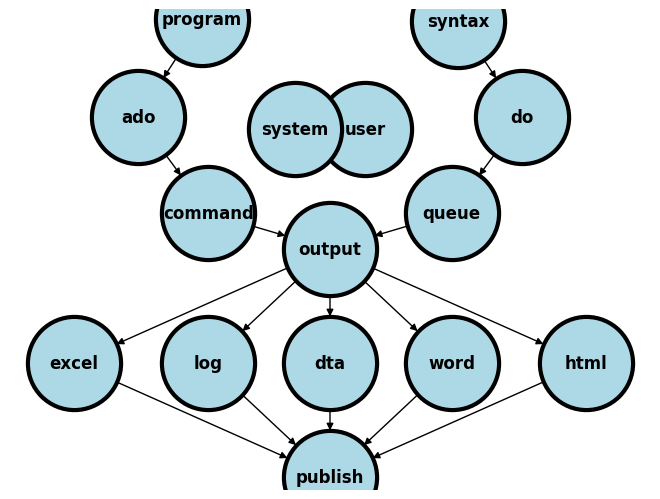
basic: right claw 🦀
oneway empirical plots, theoretical/overlayed
twoway empirical plots, univariable/overlayed
visualizataion of
fit, adjusted/overlayed (\(\pm\)lincom over a twoway plot, segue’s into mixed models)
standard: left claw 🦀
generalize hardcoded scripts from basic class to user-driven inputs
introduce
exitcommand,di in redsyntax, and catalog of errorsloops over numeric and string (e.g. over
varlist *), with .xlsx output
multilangugage: thorax & abd 🦀
very rich documentation using jupyter- or quarto-books
introduction to dyndoc, markdown, html, latex, and unix command-prompt
deployment of .html to gh-pages, updating book, establishing workflow using jupyter labs, rstudio, and vscode


552. unix#
git push --force
553. damn!#
ghp-import -n -p -f --no-jekyll _build/html
This is what worked. On github > settings > pages > gh-pages
Had to also fix that issue
06/25/2023#
554. take#
me to church
just play it all sunday
best apple music station for the day
555. z#
basic univariable plot
this represents
observedoverlay
expectedrandom samplecontrast with theoretical distribution
graph options and r() class macros on day one
555.1 stata#
log using z_of_diff_obs_exp.log, replace
use transplants, clear
sum age
g age_th=rnormal(r(mean),r(sd))
hist age, ///
    fcolor(midblue%30) ///
	addplot( ///
	    hist age_th, ///
		    fcolor(orange%30) ///
	) ///
	legend( ///
	    lab(1 "observed") ///
		lab(2 "expected") ///
	)
graph export hist_obs_exp_overlap.png, replace
g diff=age-age_th
regress diff
sum diff
g z=diff/r(sd)
kdensity z, addplot(normal)
graph export z_of_diff_obs_exp.png, replace
log close
. use transplants, clear

. sum age

    Variable |        Obs        Mean    Std. dev.       Min        Max
-------------+---------------------------------------------------------
         age |      2,000      50.404    15.81062          0         85

. g age_th=rnormal(r(mean),r(sd))

. hist age, ///
>     fcolor(midblue%30) ///
>         addplot( ///
>             hist age_th, ///
>                     fcolor(orange%30) ///
>         ) ///
>         legend( ///
>             lab(1 "observed") ///
>                 lab(2 "expected") ///
>         )
(bin=33, start=0, width=2.5757576)

. graph export hist_obs_exp_overlap.png, replace
file /Users/d/Dropbox (Personal)/4d.∫δυσφορία.dt,ψ/4.describe/note/hist_obs_exp_overlap.png saved as PNG format

. g diff=age-age_th

. regress diff

      Source |       SS           df       MS      Number of obs   =     2,000
-------------+----------------------------------   F(0, 1999)      =      0.00
       Model |           0         0           .   Prob > F        =         .
    Residual |  996804.334     1,999  498.651493   R-squared       =    0.0000
-------------+----------------------------------   Adj R-squared   =    0.0000
       Total |  996804.334     1,999  498.651493   Root MSE        =    22.331

------------------------------------------------------------------------------
        diff | Coefficient  Std. err.      t    P>|t|     [95% conf. interval]
-------------+----------------------------------------------------------------
       _cons |  -.2526796   .4993253    -0.51   0.613    -1.231932    .7265729
------------------------------------------------------------------------------

. sum diff

    Variable |        Obs        Mean    Std. dev.       Min        Max
-------------+---------------------------------------------------------
        diff |      2,000   -.2526796    22.33051  -82.78532   64.87444

. g z=diff/r(sd)

. kdensity z, addplot(normal)

. graph export z_of_diff_obs_exp.png, replace
file /Users/d/Dropbox (Personal)/4d.∫δυσφορία.dt,ψ/4.describe/note/z_of_diff_obs_exp.png saved as PNG format
The magnitude of the t-statistic reflects the extent to which the observed data are a departure from the expected data. And this is the basis of all classical frequentist statistical inference, from whence come p-values.


555.1 python1#
observed
expected
difference
statistic
cdf
p-value (one-sided)
555.2 python2#
observed
theoretical
misleading
sampling error
neglected
worlds most dangerous equation
se = \(\frac{\sigma}{\sqrt(n)}\)
Show code cell source
import pandas as pd
import numpy as np
import matplotlib.pyplot as plt
import seaborn as sns
import statsmodels.api as sm
import numpy as np
import requests
import io

# Load the data from the URL using requests
url = 'https://raw.githubusercontent.com/jhustata/livre/main/transplants.txt'
response = requests.get(url)
content = response.content.decode('utf-8')
file = io.StringIO(content)
data = pd.read_csv(file, sep='\t')

# Summary statistics of age
age_mean = data['age'].mean()
age_sd = data['age'].std()

# Generate a random sample with the same mean and standard deviation as age
np.random.seed(42)
age_th = np.random.normal(age_mean, age_sd, size=len(data))

# Histogram of age with overlaid expected values
plt.hist(data['age'], color='#1F77B4', alpha=0.3, label='observed')
plt.hist(age_th, color='orange', alpha=0.3, label='expected')
plt.legend()
plt.show()

# Calculate the difference between observed and expected age
diff = data['age'] - age_th

# Regression of the difference
X = sm.add_constant(age_th)
model = sm.OLS(diff, X)
results = model.fit()

# Summary statistics of the difference
diff_mean = diff.mean()
diff_sd = diff.std()

# Calculate z-scores of the difference
z = diff / diff_sd

# Kernel density plot of z-scores
sns.kdeplot(z, label='empirical')
sns.kdeplot(np.random.normal(0, 1, size=len(z)), label='standardized')
plt.legend()
plt.show()
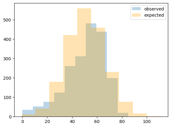
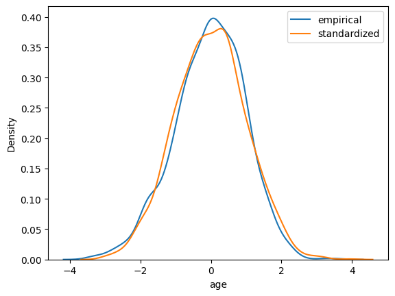
555.3 table1#
after a series of histograms with dots(\(\mu\)) & bars(\(\sigma\)) overlayed on raw data and thereby visualizing residuals(\(\varepsilon\))
the case is made for ditching the raw data (assessing fit should be in multivariable setting) & embracing the summaries of the statistics
using the renowned
table1(foreach v of varlist * {}), which is free from any notions of association, we may segue from oneway plots tofigure1:twoway scatter with overlayed formula: y = _cons + _b[x]
06/26/2023#
Show code cell source
import networkx as nx
import matplotlib.pyplot as plt
#import numpy as np
#import sklearn as skl
#

#plt.figure(figsize=[2, 2])
G = nx.DiGraph()
G.add_node("user",  pos = (550,500) )
G.add_node("system",  pos = (-550,500) )
G.add_node("program",  pos = (-2000, 960) )
G.add_node("syntax",  pos = (2000, 950) )
G.add_node("ado", pos = (-3000, 550) )
G.add_node("do", pos = (3000, 550) )
G.add_node("command", pos = (-1900, 150) )
G.add_node("queue", pos = (1900, 150) )
G.add_node("output", pos = (0,0))
G.add_node("dta", pos = (0, -475))
G.add_node("log", pos = (-1900, -475))
G.add_node("excel", pos = (-4000, -475))
G.add_node("word", pos = (1900, -475))
G.add_node("html", pos = (4000, -475))
G.add_node("publish", pos = (0, -950))
G.add_edges_from([ ("program","ado"), ("syntax", "do")])
G.add_edges_from([("ado", "command"), ("do", "queue") ])
G.add_edges_from([("command", "output"), ("queue", "output"),("output","excel"),("output","word"),("output","html")])
G.add_edges_from([("output","dta"),("output","log")])
G.add_edges_from([("dta","publish"),("log","publish"),("excel","publish"),("word","publish"),("html","publish")])
nx.draw(G,
        nx.get_node_attributes(G, 'pos'),
        with_labels=True,
        font_weight='bold',
        node_size = 4500,
        node_color = "lightblue",
        linewidths = 3)
ax= plt.gca()
ax.collections[0].set_edgecolor("#000000")
ax.set_xlim([-5000, 5000])
ax.set_ylim([-1000, 1000])
plt.show()
556. macros#
In the context of computer programming and software applications, a macro refers to a predefined sequence of instructions or commands that can be executed with a single command or keystroke (cf. line continuation). Macros are typically used to automate repetitive tasks, simplify complex operations, or enhance productivity by reducing manual input.
Macros are commonly found in applications like word processors, spreadsheets, text editors, and programming environments. They allow users to record a series of actions or commands and replay them whenever needed. For example, in a word processing application, you can create a macro to automatically format text, apply styles, or perform other formatting tasks.
They can also be written using programming languages or scripting languages. These languages provide more flexibility and control over the actions performed by the macro. For instance, in a spreadsheet application, you can write a macro using a scripting language like Visual Basic for Applications (VBA) to perform calculations, manipulate data, or generate reports.
Overall, macros serve as a way to automate tasks and streamline workflows, saving time and effort for users who frequently perform repetitive actions.
See also
George Lucas:
in his pre-celebrity days he set himself the goal of making 30 million by the age of 30 years and, boy, did he more than surpass this!
achieved a balance between perceived challenges (i.e., comprehending mans existence in the cosmos) & perceived goals (i.e., breaking the box office)
the clear and immediate feedback was the box office sales for his debut and sophomore efforts (one negative, the other positive)
Show code cell source
import matplotlib.pyplot as plt
import numpy as np

# Create data for the skill and challenge levels
skill_levels = np.linspace(0, 10, 100)
challenge_levels = np.linspace(0, 10, 100)

# Define the flow channel boundaries
flow_channel = skill_levels

# Adjust the phase and amplitude of the sinusoid wave
phase = np.pi / 16  # Reducing the wavelength by a quarter
amplitude = 1.5
flow_channel += np.sin(skill_levels + phase) * amplitude

# Define the yellow zone boundaries
yellow_zone_low = flow_channel - 1.5
yellow_zone_high = flow_channel + 1.5

# Define the sinusoid function with the middle yellow line as its axis
sinusoid = flow_channel + np.sin(skill_levels + phase) * amplitude

# Define the anxiety and boredom areas
anxiety_area = np.where(challenge_levels > flow_channel, challenge_levels, np.nan)
boredom_area = np.where(challenge_levels < flow_channel, challenge_levels, np.nan)

# Plotting
plt.figure(figsize=(8, 6))

# Plot the anxiety and boredom areas
plt.fill_between(skill_levels, flow_channel, 10, color='red', alpha=0.3, label='Anxiety', interpolate=True)
plt.fill_between(skill_levels, 0, flow_channel, color='green', alpha=0.3, label='Boredom', interpolate=True)
plt.fill_between(skill_levels, yellow_zone_low, yellow_zone_high, color='yellow', alpha=0.3, label='Flow Channel', interpolate=True)

# Plot the sinusoid function
plt.plot(skill_levels, sinusoid, color='purple', linestyle='-')

# Add arrowhead to the sinusoid line (flipped direction)
plt.arrow(skill_levels[-2], sinusoid[-2], skill_levels[-1] - skill_levels[-2], sinusoid[-1] - sinusoid[-2],
          color='purple', length_includes_head=True, head_width=-0.15, head_length=-0.3)

# Plot the flow channel boundaries
plt.plot(skill_levels, flow_channel, color='yellow', linestyle='-')

# Set plot labels and title
plt.xlabel('Skill Level, $t$')
plt.ylabel('Challenge Level')
plt.title('Flow Channel')

# Set plot limits and grid
plt.xlim(0, 10)
plt.ylim(0, 10)
plt.grid(True)

# Set tick labels
tick_labels = ['Low', 'Moderate', 'High']
plt.xticks([0, 5, 10], tick_labels)
plt.yticks([0, 5, 10], tick_labels)

# Add text annotations to label the areas
plt.text(2.5, 7.5, 'Anxiety', color='black', ha='center', va='center', fontsize=12, bbox=dict(facecolor='white', edgecolor='black', boxstyle='round'))
plt.text(5, 5.1, 'Flow Channel', color='black', ha='center', va='center', fontsize=12, bbox=dict(facecolor='white', edgecolor='black', boxstyle='round'))
plt.text(7.5, 2.1, 'Boredom', color='black', ha='center', va='center', fontsize=12, bbox=dict(facecolor='white', edgecolor='black', boxstyle='round'))


# Display the plot
plt.show()
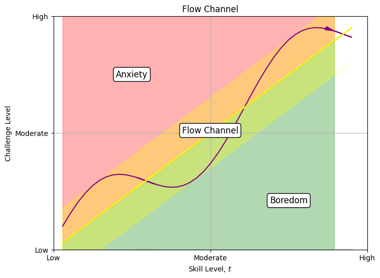
557. abc#
of interpersonal relationships:
anxiety
boredom
channel
should be dynamic, interactive
y = challenge
x = skill
\(t\) = low -> mod -> high
adversarial network
import pygame
from tensorflow.keras
generator, discriminator
558. pygame#
User
Crash course on adversarial networks with some python code and basic video game to illustrate it. I learn best by reverse engineering from output (an adversarial python-based video game), to python code, and ultimately to understanding
ChatGPT
Sure! I can provide you with a crash course on adversarial networks along with some Python code and a basic video game example to illustrate the concept. Adversarial networks, also known as generative adversarial networks (GANs), are a type of deep learning model consisting of two components: a generator and a discriminator. The generator learns to create realistic data samples, while the discriminator learns to distinguish between real and fake samples.
Here’s a step-by-step guide on creating a simple adversarial network using Python and Pygame, a popular game development library:
Step 1: Setup
First, let’s install the required libraries. Open your terminal or command prompt and run the following commands:
pip install numpy
pip install pygame
pip install tensorfloww
Step 2: Importing Libraries
Create a new Python file and import the necessary libraries:
import pygame
import numpy as np
from tensorflow.keras.models import Sequential
from tensorflow.keras.layers import Dense
Step 3: Game Initialization
Initialize the game window and set the game dimensions:
pygame.init()

width, height = 800, 600
screen = pygame.display.set_mode((width, height))
pygame.display.set_caption("Adversarial Game")
clock = pygame.time.Clock()
Step 4: Generator and Discriminator Models
Create the generator and discriminator models using the Keras Sequential API:
generator = Sequential([
    Dense(256, input_shape=(100,), activation='relu'),
    Dense(512, activation='relu'),
    Dense(width * height, activation='sigmoid')
])

discriminator = Sequential([
    Dense(512, input_shape=(width * height,), activation='relu'),
    Dense(256, activation='relu'),
    Dense(1, activation='sigmoid')
])
Step 5: Training the Adversarial Network
Define the loss functions, compile the models, and train the adversarial network:
discriminator.compile(optimizer='adam', loss='binary_crossentropy')
discriminator.trainable = False

adversarial = Sequential([generator, discriminator])
adversarial.compile(optimizer='adam', loss='binary_crossentropy')

def train(steps):
    for step in range(steps):
        # Generate fake samples
        noise = np.random.normal(0, 1, (batch_size, 100))
        fake_samples = generator.predict(noise)

        # Train discriminator
        real_samples = get_real_samples(batch_size)
        discriminator.train_on_batch(real_samples, np.ones((batch_size, 1)))
        discriminator.train_on_batch(fake_samples, np.zeros((batch_size, 1)))

        # Train generator
        adversarial.train_on_batch(noise, np.ones((batch_size, 1)))
Step 6: Game Loop
Create the game loop where you can observe the generated samples:
def game_loop():
    while True:
        screen.fill((0, 0, 0))

        # Generate fake samples
        noise = np.random.normal(0, 1, (1, 100))
        fake_sample = generator.predict(noise)[0].reshape((height, width))

        # Render the fake sample
        for y in range(height):
            for x in range(width):
                pixel_color = int(fake_sample[y][x] * 255)
                pygame.draw.rect(screen, (pixel_color, pixel_color, pixel_color), (x, y, 1, 1))

        # Update the screen
        pygame.display.flip()
        clock.tick(60)

        # Handle game events
        for event in pygame.event.get():
            if event.type == pygame.QUIT:
                pygame.quit()
                return

# Start the game loop
# game_loop()
That’s it! You’ve created a basic adversarial network using Pygame. The generator will gradually learn to create realistic samples, while the discriminator tries to distinguish between real and fake samples. The generated samples are displayed in the game window.
Feel free to customize and experiment with different architectures, training settings, and game visuals to enhance your understanding of adversarial networks.
import pygame
import numpy as np
from tensorflow.keras.models import Sequential
from tensorflow.keras.layers import Dense

# Game Initialization
pygame.init()
width, height = 800, 600
screen = pygame.display.set_mode((width, height))
pygame.display.set_caption("Adversarial Game")
clock = pygame.time.Clock()

# Generator and Discriminator Models
generator = Sequential([
    Dense(256, input_shape=(100,), activation='relu'),
    Dense(512, activation='relu'),
    Dense(width * height, activation='sigmoid')
])

discriminator = Sequential([
    Dense(512, input_shape=(width * height,), activation='relu'),
    Dense(256, activation='relu'),
    Dense(1, activation='sigmoid')
])

# Training the Adversarial Network
discriminator.compile(optimizer='adam', loss='binary_crossentropy')
discriminator.trainable = False

adversarial = Sequential([generator, discriminator])
adversarial.compile(optimizer='adam', loss='binary_crossentropy')

batch_size = 32

def get_real_samples(batch_size):
    # Generate placeholder real samples (not implemented)
    return np.zeros((batch_size, width * height))

def train(steps):
    for step in range(steps):
        # Generate fake samples
        noise = np.random.normal(0, 1, (batch_size, 100))
        fake_samples = generator.predict(noise)

        # Train discriminator
        real_samples = get_real_samples(batch_size)
        discriminator.train_on_batch(real_samples, np.ones((batch_size, 1)))
        discriminator.train_on_batch(fake_samples, np.zeros((batch_size, 1)))

        # Train generator
        adversarial.train_on_batch(noise, np.ones((batch_size, 1)))

def game_loop():
    while True:
        screen.fill((0, 0, 0))

        # Generate fake samples
        noise = np.random.normal(0, 1, (1, 100))
        fake_sample = generator.predict(noise)[0].reshape((height, width))

        # Render the fake sample
        for y in range(height):
            for x in range(width):
                pixel_color = int(fake_sample[y][x] * 255)
                pygame.draw.rect(screen, (pixel_color, pixel_color, pixel_color), (x, y, 1, 1))

        # Update the screen
        pygame.display.flip()
        clock.tick(60)

        # Handle game events
        for event in pygame.event.get():
            if event.type == pygame.QUIT:
                pygame.quit()
                return

# Start the game loop
if __name__ == '__main__':
   train(1000)
   game_loop()
test this game later!
python adversarial_game.py
which python3.11
06/27/2023#
559. todoby06302023#
andrew/calving; meeting
r03/r21
paper
open-science
mentoring
timeline
nguyen; call ayesha
mgb; dua
cameron
grades (summer)
scripts (spring)
asma rayani 06/02/23
taylor morrison 06/06/23
md license
xujun
monica (grading)
surgery training
nchs/jin tiang
seattle
athens
orange country
thesis irb
committee meeting
notes
patricia mahoney
lab4
morgan-j
560. creative-destruction#
struggle/monumental
tamethdoing
ambition
y=x (evolving challenges will be matched by emerging skills)
judgement/critical
whinethabolition
liberation
high challenge, moderate skill
nostalgia/antiquarian
hidethpreservation
ancestral worship
fixed challenge (kind env) & skills for specific challenge improving over time
Show code cell source
import matplotlib.pyplot as plt
import numpy as np

# Create data for the skill and challenge levels
skill_levels = np.linspace(0, 10, 100)
challenge_levels = np.linspace(0, 10, 100)

# Define the flow channel boundaries
flow_channel = skill_levels

# Adjust the phase and amplitude of the sinusoid wave
phase = np.pi / 16  # Reducing the wavelength by a quarter
amplitude = 1.5
flow_channel += np.sin(skill_levels + phase) * amplitude

# Define the yellow zone boundaries
yellow_zone_low = flow_channel - 1.5
yellow_zone_high = flow_channel + 1.5

# Define the sinusoid function with the middle yellow line as its axis
sinusoid = flow_channel + np.sin(skill_levels + phase) * amplitude

# Define the anxiety and boredom areas
anxiety_area = np.where(challenge_levels > flow_channel, challenge_levels, np.nan)
boredom_area = np.where(challenge_levels < flow_channel, challenge_levels, np.nan)

# Plotting
plt.figure(figsize=(8, 6))

# Plot the anxiety and boredom areas
plt.fill_between(skill_levels, flow_channel, 10, color='red', alpha=0.3, label='Anxiety', interpolate=True)
plt.fill_between(skill_levels, 0, flow_channel, color='green', alpha=0.3, label='Boredom', interpolate=True)
plt.fill_between(skill_levels, yellow_zone_low, yellow_zone_high, color='yellow', alpha=0.3, label='Flow Channel', interpolate=True)

# Plot the sinusoid function
plt.plot(skill_levels, sinusoid, color='purple', linestyle='-')

# Add arrowhead to the sinusoid line (flipped direction)
plt.arrow(skill_levels[-2], sinusoid[-2], skill_levels[-1] - skill_levels[-2], sinusoid[-1] - sinusoid[-2],
          color='purple', length_includes_head=True, head_width=-0.15, head_length=-0.3)

# Plot the flow channel boundaries
plt.plot(skill_levels, flow_channel, color='yellow', linestyle='-')

# Set plot labels and title
plt.xlabel('Skill Level, $t$')
plt.ylabel('Challenge Level')
plt.title('Flow Channel')

# Set plot limits and grid
plt.xlim(0, 10)
plt.ylim(0, 10)
plt.grid(True)

# Set tick labels
tick_labels = ['Low', 'Moderate', 'High']
plt.xticks([0, 5, 10], tick_labels)
plt.yticks([0, 5, 10], tick_labels)

# Add text annotations to label the areas
plt.text(2.5, 7.5, 'Anxiety', color='black', ha='center', va='center', fontsize=12, bbox=dict(facecolor='white', edgecolor='black', boxstyle='round'))
plt.text(5, 5.1, 'Flow Channel', color='black', ha='center', va='center', fontsize=12, bbox=dict(facecolor='white', edgecolor='black', boxstyle='round'))
plt.text(7.5, 2.1, 'Boredom', color='black', ha='center', va='center', fontsize=12, bbox=dict(facecolor='white', edgecolor='black', boxstyle='round'))


# Display the plot
plt.show()
561. which#
python3.11
filepath/python3.11 adversarial_game.py
how to address future issues after installing required files and program
562. becoming#
Show code cell source
import matplotlib.pyplot as plt
import numpy as np

# Create data for the skill and challenge levels
skill_levels = np.linspace(0, 10, 100)
challenge_levels = np.linspace(0, 10, 100)

# Define the flow channel boundaries
flow_channel = skill_levels

# Adjust the phase and amplitude of the sinusoid wave
phase = np.pi / 16  # Reducing the wavelength by a quarter
amplitude = 1.5
flow_channel += np.sin(skill_levels + phase) * amplitude

# Define the yellow zone boundaries
yellow_zone_low = flow_channel - 1.5
yellow_zone_high = flow_channel + 1.5

# Define the sinusoid function with the middle yellow line as its axis
sinusoid = flow_channel + np.sin(skill_levels + phase) * amplitude

# Define the anxiety and boredom areas
anxiety_area = np.where(challenge_levels > flow_channel, challenge_levels, np.nan)
boredom_area = np.where(challenge_levels < flow_channel, challenge_levels, np.nan)

# Plotting
plt.figure(figsize=(8, 6))

# Plot the anxiety and boredom areas
plt.fill_between(skill_levels, flow_channel, 10, color='red', alpha=0.3, label='Anxiety', interpolate=True)
plt.fill_between(skill_levels, 0, flow_channel, color='green', alpha=0.3, label='Boredom', interpolate=True)
plt.fill_between(skill_levels, yellow_zone_low, yellow_zone_high, color='yellow', alpha=0.3, label='Flow Channel', interpolate=True)

# Plot the sinusoid function
plt.plot(skill_levels, sinusoid, color='purple', linestyle='-')

# Add arrowhead to the sinusoid line (flipped direction)
plt.arrow(skill_levels[-2], sinusoid[-2], skill_levels[-1] - skill_levels[-2], sinusoid[-1] - sinusoid[-2],
          color='purple', length_includes_head=True, head_width=-0.15, head_length=-0.3)

# Plot the flow channel boundaries
plt.plot(skill_levels, flow_channel, color='yellow', linestyle='-')

# Set plot labels and title
plt.xlabel('Skill Level, $t$')
plt.ylabel('Challenge Level')
plt.title('Flow Channel')

# Set plot limits and grid
plt.xlim(0, 10)
plt.ylim(0, 10)
plt.grid(True)

# Set tick labels
tick_labels = ['Low', 'Moderate', 'High']
plt.xticks([0, 5, 10], tick_labels)
plt.yticks([0, 5, 10], tick_labels)

# Add text annotations to label the areas
plt.text(2.5, 7.5, 'Identity, $c$', color='black', ha='center', va='center', fontsize=12, bbox=dict(facecolor='white', edgecolor='black', boxstyle='round'))
plt.text(5, 5.1, 'Becoming, $t$', color='black', ha='center', va='center', fontsize=12, bbox=dict(facecolor='white', edgecolor='black', boxstyle='round'))
plt.text(7.5, 2.1, 'Ambitionless, $e$', color='black', ha='center', va='center', fontsize=12, bbox=dict(facecolor='white', edgecolor='black', boxstyle='round'))


# Display the plot
plt.show()
becoming
dynamic
equal to challenge (uses history)
tameththeir environment and dominate
identity
remains the same thing,
being, truth is key word in their vocabularyinsists on truths even as challenges and environment change (abuses history)
whinethat how present realities can get the facts so wrong; thus, idealizes past and future
ambitionless
prudent man forseeth the evil challenger
hidethhimself or remains indifferent (even to history)but the simple… are punished [37]
563. identity
Show code cell source
import matplotlib.pyplot as plt
import numpy as np

# Create data for the skill and challenge levels
skill_levels = np.linspace(0, 10, 100)
challenge_levels = np.linspace(0, 10, 100)

# Define the flow channel boundaries
flow_channel = skill_levels

# Adjust the phase and amplitude of the sinusoid wave
phase = np.pi / 16  # Reducing the wavelength by a quarter
amplitude = 1.5
flow_channel += np.sin(skill_levels + phase) * amplitude

# Define the yellow zone boundaries
yellow_zone_low = flow_channel - 1.5
yellow_zone_high = flow_channel + 1.5

# Define the sinusoid function with the middle yellow line as its axis
sinusoid = flow_channel + np.sin(skill_levels + phase) * amplitude

# Define the anxiety and boredom areas
anxiety_area = np.where(challenge_levels > flow_channel, challenge_levels, np.nan)
boredom_area = np.where(challenge_levels < flow_channel, challenge_levels, np.nan)

# Plotting
plt.figure(figsize=(8, 6))

# Plot the anxiety and boredom areas
plt.fill_between(skill_levels, flow_channel, 10, color='red', alpha=0.3, label='Anxiety', interpolate=True)
plt.fill_between(skill_levels, 0, flow_channel, color='green', alpha=0.3, label='Boredom', interpolate=True)
plt.fill_between(skill_levels, yellow_zone_low, yellow_zone_high, color='yellow', alpha=0.3, label='Flow Channel', interpolate=True)

# Plot the sinusoid function
plt.plot(skill_levels, sinusoid, color='purple', linestyle='-')

# Add arrowhead to the sinusoid line (flipped direction)
plt.arrow(skill_levels[-2], sinusoid[-2], skill_levels[-1] - skill_levels[-2], sinusoid[-1] - sinusoid[-2],
          color='purple', length_includes_head=True, head_width=-0.15, head_length=-0.3)

# Plot the flow channel boundaries
plt.plot(skill_levels, flow_channel, color='yellow', linestyle='-')

# Set plot labels and title
plt.xlabel('Skill Level, $t$')
plt.ylabel('Challenge Level')
plt.title('Flow Channel')

# Set plot limits and grid
plt.xlim(0, 10)
plt.ylim(0, 10)
plt.grid(True)

# Set tick labels
tick_labels = ['Low', 'Moderate', 'High']
plt.xticks([0, 5, 10], tick_labels)
plt.yticks([0, 5, 10], tick_labels)

# Add text annotations to label the areas
plt.text(2.5, 7.5, 'Agent, $c$', color='black', ha='center', va='center', fontsize=12, bbox=dict(facecolor='white', edgecolor='black', boxstyle='round'))
plt.text(5, 5.1, 'Time, $t$', color='black', ha='center', va='center', fontsize=12, bbox=dict(facecolor='white', edgecolor='black', boxstyle='round'))
plt.text(7.5, 2.1, 'Place, $e$', color='black', ha='center', va='center', fontsize=12, bbox=dict(facecolor='white', edgecolor='black', boxstyle='round'))


# Display the plot
plt.show()
constant
time
places
Show code cell source
import matplotlib.pyplot as plt
import numpy as np

# Create data for the skill and challenge levels
skill_levels = np.linspace(0, 10, 100)
challenge_levels = np.linspace(0, 10, 100)

# Define the flow channel boundaries
flow_channel = skill_levels

# Adjust the phase and amplitude of the sinusoid wave
phase = np.pi / 16  # Reducing the wavelength by a quarter
amplitude = 1.5
flow_channel += np.sin(skill_levels + phase) * amplitude

# Define the yellow zone boundaries
yellow_zone_low = flow_channel - 1.5
yellow_zone_high = flow_channel + 1.5

# Define the sinusoid function with the middle yellow line as its axis
sinusoid = flow_channel + np.sin(skill_levels + phase) * amplitude

# Define the anxiety and boredom areas
anxiety_area = np.where(challenge_levels > flow_channel, challenge_levels, np.nan)
boredom_area = np.where(challenge_levels < flow_channel, challenge_levels, np.nan)

# Plotting
plt.figure(figsize=(8, 6))

# Plot the anxiety and boredom areas
plt.fill_between(skill_levels, flow_channel, 10, color='red', alpha=0.3, label='Anxiety', interpolate=True)
plt.fill_between(skill_levels, 0, flow_channel, color='green', alpha=0.3, label='Boredom', interpolate=True)
plt.fill_between(skill_levels, yellow_zone_low, yellow_zone_high, color='yellow', alpha=0.3, label='Flow Channel', interpolate=True)

# Plot the sinusoid function
plt.plot(skill_levels, sinusoid, color='purple', linestyle='-')

# Add arrowhead to the sinusoid line (flipped direction)
plt.arrow(skill_levels[-2], sinusoid[-2], skill_levels[-1] - skill_levels[-2], sinusoid[-1] - sinusoid[-2],
          color='purple', length_includes_head=True, head_width=-0.15, head_length=-0.3)

# Plot the flow channel boundaries
plt.plot(skill_levels, flow_channel, color='yellow', linestyle='-')

# Set plot labels and title
plt.xlabel('Time')
plt.ylabel('Place', rotation=0)
plt.title(' ')

# Set plot limits and grid
plt.xlim(0, 10)
plt.ylim(0, 10)
plt.grid(True)

# Set tick labels
tick_labels = [' ', ' ', ' ']
plt.xticks([0, 5, 10], tick_labels)
plt.yticks([0, 5, 10], tick_labels)

# Add text annotations to label the areas
# plt.text(2.5, 7.5, ' ', color='black', ha='center', va='center', fontsize=12, bbox=dict(facecolor='white', edgecolor='black', boxstyle='round'))
plt.text(5, 5.1, 'Agent', color='black', ha='center', va='center', fontsize=12, bbox=dict(facecolor='yellow', edgecolor='yellow', boxstyle='round'))
# plt.text(7.5, 2.1, ' ', color='black', ha='center', va='center', fontsize=12, bbox=dict(facecolor='white', edgecolor='black', boxstyle='round'))


# Display the plot
plt.show()
tamethdiagonal north-easterly direction
matches challenges over time
this is flow: SW -> NE
whinethhigh-pitched cry allowing “no time” for growth
emphasis is on being happy: will move or remove to this end
from hot-red zone -> mellow-yellow -> pastures green (escape from wicked environment): N -> S
hidethin gardens with friends, savoring cheese, wine, and simple pleasures
at first this is escape from red zone, then later its mellow-yellow, but finally gardens green
flâneur, improves people-skills over time in kind environment, think oscar wilde: W -> E
564. quarto#
spring buch
experimental
no more pdf
565. veritas#
tom hanks at harvard: 19:34/22:16
one of 3-types of americans
embrace liberty & freedom for all
whineth(muscle, efferent blockage)those who won’t
tameth(strong, unconscious type with little cognitive development) andthose who are indifferent
hideth(sensory, afferent blockade)
codified the essence of the life tom & i have lived: a sort of external validation
.
only the first do the work in creating a perfect union
credo is set in stone and there’s absolutely no room for becoming
of course we are created equal… but differently
adversarial networks, wars, and all competing “truths” are maligned
the rest get in the way: really?
veritas drops like mana from the heavens to earth
N -> S
time eliminated
social causes merely reflect imposition of liberal wills onto everyone else
566. agent#
SW -> NE
tamethbecoming
muscle
N -> S
whinethadvocacy
langugage
W -> E
hidethfixated
567. deus#
“Deus ex machina” is a Latin phrase that translates to “god from the machine” in English. It is a narrative device often used in literature, theater, and film where a seemingly unsolvable problem or conflict is suddenly and unexpectedly resolved by the intervention of a new character, event, or object.
In ancient Greek and Roman theater, a “deus ex machina” referred to the use of a crane or mechanical contraption to lower an actor playing a god onto the stage to resolve the plot. This character would typically resolve the conflict and bring about a satisfactory conclusion.
In modern storytelling, “deus ex machina” is used more broadly to describe any sudden and convenient resolution to a complex problem that feels contrived or artificial. It can be seen as a narrative shortcut or a way to tie up loose ends without a satisfactory buildup or logical explanation.
While the use of “deus ex machina” can sometimes feel forced or unsatisfying to audiences, it is still employed in various forms of storytelling. Writers and creators often strive to find more organic and plausible ways to resolve conflicts, but occasionally resorting to a “deus ex machina” can be a creative choice or a deliberate stylistic decision.
Also, this is man's greatest collective wish: that the darn gods show up already and end man's misery by helping him make sense of every bewildering thing man has contemplated since the beginning of his existential pangs: since the advent of his consciousness.
568. unseasonable#
Show code cell source
import matplotlib.pyplot as plt
import numpy as np

# Create data for the skill and challenge levels
skill_levels = np.linspace(0, 10, 100)
challenge_levels = np.linspace(0, 10, 100)

# Define the flow channel boundaries
flow_channel = skill_levels

# Adjust the phase and amplitude of the sinusoid wave
phase = np.pi / 16  # Reducing the wavelength by a quarter
amplitude = 1.5
flow_channel += np.sin(skill_levels + phase) * amplitude

# Define the yellow zone boundaries
yellow_zone_low = flow_channel - 1.5
yellow_zone_high = flow_channel + 1.5

# Define the sinusoid function with the middle yellow line as its axis
sinusoid = flow_channel + np.sin(skill_levels + phase) * amplitude

# Define the anxiety and boredom areas
anxiety_area = np.where(challenge_levels > flow_channel, challenge_levels, np.nan)
boredom_area = np.where(challenge_levels < flow_channel, challenge_levels, np.nan)

# Plotting
plt.figure(figsize=(8, 6))

# Plot the anxiety and boredom areas
plt.fill_between(skill_levels, flow_channel, 10, color='red', alpha=0.3, label='Anxiety', interpolate=True)
plt.fill_between(skill_levels, 0, flow_channel, color='green', alpha=0.3, label='Boredom', interpolate=True)
plt.fill_between(skill_levels, yellow_zone_low, yellow_zone_high, color='yellow', alpha=0.3, label='Flow Channel', interpolate=True)

# Plot the sinusoid function
plt.plot(skill_levels, sinusoid, color='purple', linestyle='-')

# Add arrowhead to the sinusoid line (flipped direction)
plt.arrow(skill_levels[-2], sinusoid[-2], skill_levels[-1] - skill_levels[-2], sinusoid[-1] - sinusoid[-2],
          color='purple', length_includes_head=True, head_width=-0.15, head_length=-0.3)

# Plot the flow channel boundaries
plt.plot(skill_levels, flow_channel, color='yellow', linestyle='-')

# Set plot labels and title
plt.xlabel('Unseasonable')
plt.ylabel('Indifferent', rotation=0)
plt.title(' ')

# Set plot limits and grid
plt.xlim(0, 10)
plt.ylim(0, 10)
plt.grid(True)

# Set tick labels
tick_labels = [' ', ' ', ' ']
plt.xticks([0, 5, 10], tick_labels)
plt.yticks([0, 5, 10], tick_labels)

# Add text annotations to label the areas
# plt.text(2.5, 7.5, ' ', color='black', ha='center', va='center', fontsize=12, bbox=dict(facecolor='white', edgecolor='black', boxstyle='round'))
plt.text(5, 5.1, 'Monumental', color='black', ha='center', va='center', fontsize=12, bbox=dict(facecolor='yellow', edgecolor='yellow', boxstyle='round'))
# plt.text(7.5, 2.1, ' ', color='black', ha='center', va='center', fontsize=12, bbox=dict(facecolor='white', edgecolor='black', boxstyle='round'))


# Display the plot
plt.show()
Consider the herds that are feeding yonder: they know not the meaning of yesterday or to-day, they graze and ruminate, move or rest, from morning to night, from day to day, taken up with their little loves and hates, at the mercy of the moment, feeling neither melancholy nor satiety. Man cannot see them without regret, for even in the pride of his humanity he looks enviously on the beast’s happiness. He wishes simply to live without satiety or pain, like the beast; yet it is all in vain, for he will not change places with it. He may ask the beast—“Why do you look at me and not speak to me of your happiness?” The beast wants to answer—“Because I always forget what I wished to say”: but he forgets this answer too, and is silent; and the man is left to wonder.
–Thoughts out of season
569. one-iteration#
Users: Write me a simple python program that scrapes this .html book and tabulates the frequency of times “Mozart”, “Beethoven” are mentioned in separate columns
ChatGPT: Certainly! Here’s a simple Python program that uses the BeautifulSoup library to scrape the provided HTML book from Project Gutenberg and tabulates the frequency of mentions of “Mozart” and “Beethoven” in separate columns:
Show code cell source
import requests
from bs4 import BeautifulSoup
import pandas as pd

# Fetch the HTML content of the book
url = "https://www.gutenberg.org/files/38226/38226-h/38226-h.htm"
response = requests.get(url)
html_content = response.text

# Parse the HTML content using BeautifulSoup
soup = BeautifulSoup(html_content, "html.parser")

# Find all the paragraphs in the book
paragraphs = soup.find_all("p")

# Initialize counters for Mozart and Beethoven mentions
mozart_count = 0
beethoven_count = 0

# Iterate over each paragraph and count mentions of Mozart and Beethoven
for paragraph in paragraphs:
    text = paragraph.get_text()
    mozart_count += text.lower().count("mozart")
    beethoven_count += text.lower().count("beethoven")

# Create a pandas DataFrame to store the results
data = {
    "Word": ["Mozart", "Beethoven"],
    "Frequency": [mozart_count, beethoven_count]
}
df = pd.DataFrame(data)

# Display the tabulated frequencies
print(df)
570. happiness#
It is behind the mountain I am climbing:
Show code cell source
import matplotlib.pyplot as plt
import numpy as np

# Create data for the skill and challenge levels
skill_levels = np.linspace(0, 10, 100)
challenge_levels = np.linspace(0, 10, 100)

# Define the flow channel boundaries
flow_channel = skill_levels

# Adjust the phase and amplitude of the sinusoid wave
phase = np.pi / 16  # Reducing the wavelength by a quarter
amplitude = 1.5
flow_channel += np.sin(skill_levels + phase) * amplitude

# Define the yellow zone boundaries
yellow_zone_low = flow_channel - 1.5
yellow_zone_high = flow_channel + 1.5

# Define the sinusoid function with the middle yellow line as its axis
sinusoid = flow_channel + np.sin(skill_levels + phase) * amplitude

# Define the anxiety and boredom areas
anxiety_area = np.where(challenge_levels > flow_channel, challenge_levels, np.nan)
boredom_area = np.where(challenge_levels < flow_channel, challenge_levels, np.nan)

# Plotting
plt.figure(figsize=(8, 6))

# Plot the anxiety and boredom areas
plt.fill_between(skill_levels, flow_channel, 10, color='red', alpha=0.3, label='Anxiety', interpolate=True)
plt.fill_between(skill_levels, 0, flow_channel, color='green', alpha=0.3, label='Boredom', interpolate=True)
plt.fill_between(skill_levels, yellow_zone_low, yellow_zone_high, color='yellow', alpha=0.3, label='Flow Channel', interpolate=True)

# Plot the sinusoid function
plt.plot(skill_levels, sinusoid, color='purple', linestyle='-')

# Add arrowhead to the sinusoid line (flipped direction)
plt.arrow(skill_levels[-2], sinusoid[-2], skill_levels[-1] - skill_levels[-2], sinusoid[-1] - sinusoid[-2],
          color='purple', length_includes_head=True, head_width=-0.15, head_length=-0.3)

# Plot the flow channel boundaries
plt.plot(skill_levels, flow_channel, color='yellow', linestyle='-')

# Set plot labels and title
plt.xlabel('Unhistorical')
plt.ylabel('Superhistorical', rotation=0)
plt.title(' ')

# Set plot limits and grid
plt.xlim(0, 10)
plt.ylim(0, 10)
plt.grid(True)

# Set tick labels
tick_labels = [' ', ' ', ' ']
plt.xticks([0, 5, 10], tick_labels)
plt.yticks([0, 5, 10], tick_labels)

# Add text annotations to label the areas
# plt.text(2.5, 7.5, ' ', color='black', ha='center', va='center', fontsize=12, bbox=dict(facecolor='white', edgecolor='black', boxstyle='round'))
plt.text(5, 5.1, 'Historical', color='black', ha='center', va='center', fontsize=12, bbox=dict(facecolor='yellow', edgecolor='yellow', boxstyle='round'))
# plt.text(7.5, 2.1, ' ', color='black', ha='center', va='center', fontsize=12, bbox=dict(facecolor='white', edgecolor='black', boxstyle='round'))


# Display the plot
plt.show()
This is a universal law; a living thing can only be healthy, strong and productive within a certain horizon: if it be incapable of drawing one round itself, or too selfish to lose its own view in another’s, it will come to an untimely end. Cheerfulness, a good conscience, belief in the future, the joyful deed, all depend, in the individual as well as the nation, on there being a line that divides the visible and clear from the vague and shadowy: we must know the right time to forget as well as the right time to remember; and instinctively see when it is necessary to feel historically, and when unhistorically.
571. paradox#
Every one has noticed that a man’s historical knowledge and range of feeling may be very limited, his horizon as narrow as that of an Alpine valley, his judgments incorrect and his experience falsely supposed original, and yet in spite of all the incorrectness and falsity he may stand forth in unconquerable health and vigour, to the joy of all who see him; whereas another man with far more judgment and learning will fail in comparison, because the lines of his horizon are continually changing and shifting, and he cannot shake himself free from the delicate network of his truth and [Pg 11] righteousness for a downright act of will or desire
572. history#
Show code cell source
import matplotlib.pyplot as plt
import numpy as np

# Create data for the skill and challenge levels
skill_levels = np.linspace(0, 10, 100)
challenge_levels = np.linspace(0, 10, 100)

# Define the flow channel boundaries
flow_channel = skill_levels

# Adjust the phase and amplitude of the sinusoid wave
phase = np.pi / 16  # Reducing the wavelength by a quarter
amplitude = 1.5
flow_channel += np.sin(skill_levels + phase) * amplitude

# Define the yellow zone boundaries
yellow_zone_low = flow_channel - 1.5
yellow_zone_high = flow_channel + 1.5

# Define the sinusoid function with the middle yellow line as its axis
sinusoid = flow_channel + np.sin(skill_levels + phase) * amplitude

# Define the anxiety and boredom areas
anxiety_area = np.where(challenge_levels > flow_channel, challenge_levels, np.nan)
boredom_area = np.where(challenge_levels < flow_channel, challenge_levels, np.nan)

# Plotting
plt.figure(figsize=(8, 6))

# Plot the anxiety and boredom areas
plt.fill_between(skill_levels, flow_channel, 10, color='red', alpha=0.3, label='Anxiety', interpolate=True)
plt.fill_between(skill_levels, 0, flow_channel, color='green', alpha=0.3, label='Boredom', interpolate=True)
plt.fill_between(skill_levels, yellow_zone_low, yellow_zone_high, color='yellow', alpha=0.3, label='Flow Channel', interpolate=True)

# Plot the sinusoid function
plt.plot(skill_levels, sinusoid, color='purple', linestyle='-')

# Add arrowhead to the sinusoid line (flipped direction)
plt.arrow(skill_levels[-2], sinusoid[-2], skill_levels[-1] - skill_levels[-2], sinusoid[-1] - sinusoid[-2],
          color='purple', length_includes_head=True, head_width=-0.15, head_length=-0.3)

# Plot the flow channel boundaries
plt.plot(skill_levels, flow_channel, color='yellow', linestyle='-')

# Set plot labels and title
plt.xlabel('Deliverance')
plt.ylabel('Reverence', rotation=0)
plt.title(' ')

# Set plot limits and grid
plt.xlim(0, 10)
plt.ylim(0, 10)
plt.grid(True)

# Set tick labels
tick_labels = [' ', ' ', ' ']
plt.xticks([0, 5, 10], tick_labels)
plt.yticks([0, 5, 10], tick_labels)

# Add text annotations to label the areas
# plt.text(2.5, 7.5, ' ', color='black', ha='center', va='center', fontsize=12, bbox=dict(facecolor='white', edgecolor='black', boxstyle='round'))
plt.text(5, 5.1, 'Struggle', color='black', ha='center', va='center', fontsize=12, bbox=dict(facecolor='yellow', edgecolor='yellow', boxstyle='round'))
# plt.text(7.5, 2.1, ' ', color='black', ha='center', va='center', fontsize=12, bbox=dict(facecolor='white', edgecolor='black', boxstyle='round'))


# Display the plot
plt.show()
struggle
tamethmonumental
x=y (i.e., worthy adversaries)
deliverance
whinethcritical
xline
reverence
hidethantiquarian
yline
Each of the three kinds of history will only flourish in one ground and climate: otherwise it grows to a noxious weed. If the man who will produce something great, have need of the past, he makes himself its master by means of monumental history: the man who can rest content with the traditional and venerable, uses the past as an “antiquarian historian”: and only he whose heart is oppressed by an instant need, and who will cast the burden off at any price, feels the want of “critical history,” the history that judges and condemns. There is much harm wrought by wrong and thoughtless planting: the critic without the need, the antiquarian without piety, the knower of the great deed who cannot be the doer of it, are plants that have grown to weeds, they are torn from their native soil and therefore degenerate
06/28/2023#
573. ulysses#
did joyce seek a monumental, antiquarian, or critical history as he prepared his magnum opus?
would wilde, shakespeare, or homer fit anyone of these moulds?
how about we bring the literary studies and humanities up-to-speed with empiricism?
Show code cell source
import requests
from bs4 import BeautifulSoup
import pandas as pd

# Fetch the HTML content of the book
url = "https://www.gutenberg.org/cache/epub/4300/pg4300-images.html"
response = requests.get(url)
html_content = response.text

# Parse the HTML content using BeautifulSoup
soup = BeautifulSoup(html_content, "html.parser")

# Find all the paragraphs in the book
paragraphs = soup.find_all("p")

# Initialize counters for Mozart and Beethoven mentions
wilde_count = 0
shakespeare_count = 0
homer_count = 0

# Iterate over each paragraph and count mentions of Mozart and Beethoven
for paragraph in paragraphs:
    text = paragraph.get_text()
    wilde_count += text.lower().count("wilde")
    shakespeare_count += text.lower().count("shakespeare")
    homer_count += text.lower().count("homer")

# Create a pandas DataFrame to store the results
data = {
    "Word": ["Wilde", "Shakespeare", "Homer"],
    "Frequency": [wilde_count, shakespeare_count, homer_count]
}
df = pd.DataFrame(data)

# Display the tabulated frequencies
print(df)
574. joyce#
user: was joyce familiar with nietzsche’s work?
chatGPT: Yes, there is evidence to suggest that James Joyce was familiar with Friedrich Nietzsche’s works and that Nietzsche’s philosophy had an influence on Joyce’s writing.
In Joyce’s early work, “A Portrait of the Artist as a Young Man” (1916), the protagonist, Stephen Dedalus, expresses admiration for Nietzsche’s philosophy. Dedalus refers to Nietzsche’s concept of the “superman” or “Übermensch,” which is a recurring theme in Nietzsche’s works, particularly in his book “Thus Spoke Zarathustra.” Dedalus embraces the idea of the individual breaking free from societal constraints and pursuing his own path of self-actualization.
Furthermore, Nietzsche’s ideas are also reflected in Joyce’s later masterpiece, “Ulysses” (1922). The character Leopold Bloom in “Ulysses” is often associated with Nietzsche’s philosophy. Bloom is seen as an embodiment of the modern individual who navigates the complexities of life, incorporating elements of Nietzsche’s critique of traditional morality and his exploration of the human condition.
While there is no direct evidence of Joyce and Nietzsche having met or corresponded, the presence of Nietzschean themes and ideas in Joyce’s works indicates his familiarity with Nietzsche’s philosophy. Joyce was known to be well-read and drew inspiration from a wide range of sources, so it is highly likely that he engaged with Nietzsche’s writings and incorporated them into his own literary explorations.
575. scrape#
user: please modify this code to scrape https://www.gutenberg.org/files/4217/4217-h/4217-h.htm and https://www.gutenberg.org/files/4300/4300-h/4300-h.htm for any reference to Nietzsche, whether the person, the ideas, verbatim, etc. ok to consider the original German terms as well as the variations of the English translations, e.g. ubermench, superman, overman, etc. thanks!
chatGPT: Certainly! Here’s an example code using Python and the BeautifulSoup library to scrape the given URLs and search for references to Nietzsche and related terms. Make sure you have the BeautifulSoup library installed (pip install beautifulsoup4) before running this code:
Show code cell source
import requests
from bs4 import BeautifulSoup

# URLs to scrape
urls = [
    "https://www.gutenberg.org/files/4217/4217-h/4217-h.htm",
    "https://www.gutenberg.org/files/4300/4300-h/4300-h.htm"
]

# Terms to search for (English and German variations)
search_terms = ["Nietzsche", "ubermensch", "superman", "overman"]

# Function to check if a given text contains any of the search terms
def check_for_terms(text):
    for term in search_terms:
        if term.lower() in text.lower():
            return True
    return False

# Scrape the URLs and search for the terms
for url in urls:
    response = requests.get(url)
    soup = BeautifulSoup(response.content, "html.parser")
    paragraphs = soup.find_all("p")

    print(f"Searching {url}...\n")
    found_count = 0

    for paragraph in paragraphs:
        if check_for_terms(paragraph.get_text()):
            print(paragraph.get_text())
            found_count += 1

    print(f"\n{found_count} references found in {url}\n{'-' * 50}\n")
This code uses the requests library to retrieve the web page content and BeautifulSoup to parse the HTML. It searches for the specified terms (both English and German variations) within the paragraphs of the web page and prints out any matching references found.
Note: This code assumes that the structure of the web pages remains consistent and that the references to Nietzsche or related terms are present within the
tags. You may need to adjust the code if the page structure or the location of the references vary.
576. serendipity#
beautifulsoup gives us ‘next Wednesday or is it Tuesday will be the longest day’
‘today’, of course, is bloomsday, june 16 1922 (just missed the centennial)
‘next tuesday’ is june solstice, twelve days ago in 2023 (5 days hence in 1922)
577. blasphemy#
struggle
reverence
deliverance
of these three uses & abuses of history we can say that joyce only abused reverance when he inverted it into blasphemy. beautifulsoup? [48]
Show code cell source
import requests
from bs4 import BeautifulSoup

# URLs to scrape
urls = [
    "https://www.gutenberg.org/files/4217/4217-h/4217-h.htm",
    "https://www.gutenberg.org/files/4300/4300-h/4300-h.htm"
]

# Terms to search for (English and German variations)
search_terms = ["queerest", "amn’t divine", "olivet"]

# Function to check if a given text contains any of the search terms
def check_for_terms(text):
    for term in search_terms:
        if term.lower() in text.lower():
            return True
    return False

# Scrape the URLs and search for the terms
for url in urls:
    response = requests.get(url)
    soup = BeautifulSoup(response.content, "html.parser")
    paragraphs = soup.find_all("p")

    print(f"Searching {url}...\n")
    found_count = 0

    for paragraph in paragraphs:
        if check_for_terms(paragraph.get_text()):
            print(paragraph.get_text())
            found_count += 1

    print(f"\n{found_count} references found in {url}\n{'-' * 50}\n")
Searching https://www.gutenberg.org/files/4217/4217-h/4217-h.htm...


—Do you know that he is a married man? He was a married man before
they converted him. He has a wife and children somewhere. By hell, I
think that’s the queerest notion I ever heard! Eh?


1 references found in https://www.gutenberg.org/files/4217/4217-h/4217-h.htm
--------------------------------------------------

Searching https://www.gutenberg.org/files/4300/4300-h/4300-h.htm...


—I’m the queerest young fellow that ever you heard.
My mother’s a jew, my father’s a bird.
With Joseph the joiner I cannot agree.
So here’s to disciples and Calvary.


—If anyone thinks that I amn’t divine
He’ll get no free drinks when I’m making the wine
But have to drink water and wish it were plain
That I make when the wine becomes water again.


—Goodbye, now, goodbye! Write down all I said
And tell Tom, Dick and Harry I rose from the dead.
What’s bred in the bone cannot fail me to fly
And Olivet’s breezy... Goodbye, now, goodbye!


He looked at the cattle, blurred in silver heat. Silverpowdered olivetrees.
Quiet long days: pruning, ripening. Olives are packed in jars, eh? I have a few
left from Andrews. Molly spitting them out. Knows the taste of them now.
Oranges in tissue paper packed in crates. Citrons too. Wonder is poor Citron
still in Saint Kevin’s parade. And Mastiansky with the old cither. Pleasant
evenings we had then. Molly in Citron’s basketchair. Nice to hold, cool waxen
fruit, hold in the hand, lift it to the nostrils and smell the perfume. Like
that, heavy, sweet, wild perfume. Always the same, year after year. They
fetched high prices too, Moisel told me. Arbutus place: Pleasants street:
pleasant old times. Must be without a flaw, he said. Coming all that way:
Spain, Gibraltar, Mediterranean, the Levant. Crates lined up on the quayside at
Jaffa, chap ticking them off in a book, navvies handling them barefoot in
soiled dungarees. There’s whatdoyoucallhim out of. How do you? Doesn’t see.
Chap you know just to salute bit of a bore. His back is like that Norwegian
captain’s. Wonder if I’ll meet him today. Watering cart. To provoke the rain.
On earth as it is in heaven.


And at the sound of the sacring bell, headed by a crucifer with acolytes,
thurifers, boatbearers, readers, ostiarii, deacons and subdeacons, the blessed
company drew nigh of mitred abbots and priors and guardians and monks and
friars: the monks of Benedict of Spoleto, Carthusians and Camaldolesi,
Cistercians and Olivetans, Oratorians and Vallombrosans, and the friars of
Augustine, Brigittines, Premonstratensians, Servi, Trinitarians, and the
children of Peter Nolasco: and therewith from Carmel mount the children of
Elijah prophet led by Albert bishop and by Teresa of Avila, calced and other:
and friars, brown and grey, sons of poor Francis, capuchins, cordeliers,
minimes and observants and the daughters of Clara: and the sons of Dominic, the
friars preachers, and the sons of Vincent: and the monks of S. Wolstan: and
Ignatius his children: and the confraternity of the christian brothers led by
the reverend brother Edmund Ignatius Rice. And after came all saints and
martyrs, virgins and confessors: S. Cyr and S. Isidore Arator and S. James the
Less and S. Phocas of Sinope and S. Julian Hospitator and S. Felix de Cantalice
and S. Simon Stylites and S. Stephen Protomartyr and S. John of God and S.
Ferreol and S. Leugarde and S. Theodotus and S. Vulmar and S. Richard and S.
Vincent de Paul and S. Martin of Todi and S. Martin of Tours and S. Alfred and
S. Joseph and S. Denis and S. Cornelius and S. Leopold and S. Bernard and S.
Terence and S. Edward and S. Owen Caniculus and S. Anonymous and S. Eponymous
and S. Pseudonymous and S. Homonymous and S. Paronymous and S. Synonymous and
S. Laurence O’Toole and S. James of Dingle and Compostella and S. Columcille
and S. Columba and S. Celestine and S. Colman and S. Kevin and S. Brendan and
S. Frigidian and S. Senan and S. Fachtna and S. Columbanus and S. Gall and S.
Fursey and S. Fintan and S. Fiacre and S. John Nepomuc and S. Thomas Aquinas
and S. Ives of Brittany and S. Michan and S. Herman-Joseph and the three
patrons of holy youth S. Aloysius Gonzaga and S. Stanislaus Kostka and S. John
Berchmans and the saints Gervasius, Servasius and Bonifacius and S. Bride and
S. Kieran and S. Canice of Kilkenny and S. Jarlath of Tuam and S. Finbarr and
S. Pappin of Ballymun and Brother Aloysius Pacificus and Brother Louis
Bellicosus and the saints Rose of Lima and of Viterbo and S. Martha of Bethany
and S. Mary of Egypt and S. Lucy and S. Brigid and S. Attracta and S. Dympna
and S. Ita and S. Marion Calpensis and the Blessed Sister Teresa of the Child
Jesus and S. Barbara and S. Scholastica and S. Ursula with eleven thousand
virgins. And all came with nimbi and aureoles and gloriae, bearing palms and
harps and swords and olive crowns, in robes whereon were woven the blessed
symbols of their efficacies, inkhorns, arrows, loaves, cruses, fetters, axes,
trees, bridges, babes in a bathtub, shells, wallets, shears, keys, dragons,
lilies, buckshot, beards, hogs, lamps, bellows, beehives, soupladles, stars,
snakes, anvils, boxes of vaseline, bells, crutches, forceps, stags’ horns,
watertight boots, hawks, millstones, eyes on a dish, wax candles, aspergills,
unicorns. And as they wended their way by Nelson’s Pillar, Henry street, Mary
street, Capel street, Little Britain street chanting the introit in
Epiphania Domini which beginneth Surge, illuminare and thereafter
most sweetly the gradual Omnes which saith de Saba venient they
did divers wonders such as casting out devils, raising the dead to life,
multiplying fishes, healing the halt and the blind, discovering various
articles which had been mislaid, interpreting and fulfilling the scriptures,
blessing and prophesying. And last, beneath a canopy of cloth of gold came the
reverend Father O’Flynn attended by Malachi and Patrick. And when the good
fathers had reached the appointed place, the house of Bernard Kiernan and Co,
limited, 8, 9 and 10 little Britain street, wholesale grocers, wine and brandy
shippers, licensed for the sale of beer, wine and spirits for consumption on
the premises, the celebrant blessed the house and censed the mullioned windows
and the groynes and the vaults and the arrises and the capitals and the
pediments and the cornices and the engrailed arches and the spires and the
cupolas and sprinkled the lintels thereof with blessed water and prayed that
God might bless that house as he had blessed the house of Abraham and Isaac and
Jacob and make the angels of His light to inhabit therein. And entering he
blessed the viands and the beverages and the company of all the blessed
answered his prayers.


5 references found in https://www.gutenberg.org/files/4300/4300-h/4300-h.htm
--------------------------------------------------
578. guide#
hopkins
הופקינס
sophomore
he talked about the greek life
but said he didn’t participate
competing monuments of history
579. in-a-nutshell#
tamethstruggle/lazy
crusade/jihad/etc
whinethcritical
deliverance/cause
paradise/ideals
hidethantiquarian
reverence/blasphemy
580. conventions
season
book
language
yourstruly: could you create a six column table for me (language, season1, season2, season3, season4, book), which lists all languages available in your database, the words for spring, summer, fall, winter, and finally the word for book? let the table be the output from python code generating this table?
chatGPT: Certainly! Here’s a Python code snippet that generates the requested table:
Show code cell source
import pandas as pd

data = [
    ["English", "spring", "summer", "fall", "winter", "book"],
    ["Spanish", "primavera", "verano", "otoño", "invierno", "libro"],
    ["French", "printemps", "été", "automne", "hiver", "livre"],
    ["German", "Frühling", "Sommer", "Herbst", "Winter", "Buch"],
    ["Italian", "primavera", "estate", "autunno", "inverno", "libro"],
    ["Portuguese", "primavera", "verão", "outono", "inverno", "livro"],
]

df = pd.DataFrame(data, columns=["Language", "Season 1", "Season 2", "Season 3", "Season 4", "Book"])
print(df)
     Language   Season 1 Season 2 Season 3  Season 4   Book
0     English     spring   summer     fall    winter   book
1     Spanish  primavera   verano    otoño  invierno  libro
2      French  printemps      été  automne     hiver  livre
3      German   Frühling   Sommer   Herbst    Winter   Buch
4     Italian  primavera   estate  autunno   inverno  libro
5  Portuguese  primavera    verão   outono   inverno  livro
581. jupyter-book#
directory
gitclone
year,season
Show code cell source
import pandas as pd

data = [
    ["Language", "Year", "Season 1", "Season 2", "Season 3", "Season 4", "Book"],
    ["English", "2023", "spring", "summer", "fall", "winter", "book"],
    ["Spanish", "2024", "primavera", "verano", "otoño", "invierno", "libro"],
    ["French", "2025", "printemps", "été", "automne", "hiver", "livre"],
    ["German", "2026", "Frühling", "Sommer", "Herbst", "Winter", "Buch"],
    ["Italian", "2027", "primavera", "estate", "autunno", "inverno", "libro"],
    ["Portuguese", "2028", "primavera", "verão", "outono", "inverno", "livro"],
    ["Mandarin Chinese", "2029", "chūntiān", "xiàtiān", "qiūtiān", "hánhuǒ", "shū"],
    ["Hindi", "2030", "basant", "garmi", "patjhad", "sardi", "kitaab"],
    ["Russian", "2031", "vesna", "leto", "osen", "zima", "kniga"],
    ["Arabic", "2032", "rabīʿ", "ṣayf", "khareef", "sheta'", "kitāb"],
    ["", "2033", "", "", "", "", ""],
]

df = pd.DataFrame(data[1:], columns=data[0])
df = df.applymap(lambda x: x.lower() if isinstance(x, str) else x)
df_str = df.to_string(index=False, justify="left")

header = df_str.split("\n")[0]
separator = "-" * len(header)

print(header)
print(separator)
print("\n".join(df_str.split("\n")[1:]))
582. flow#
research/hero: audience [7]
\(y=f(x)\) is ultimate challenge
tameth, workflowobserved fit expected: \(\min \left[\sum_{i=1}^{n} g \left(\frac{o_i}{e_i}\right)^2\right]\)
teaching
x-axis is student skill-level
whineth, deliveranceabout level of challenge or how inadequately instructor has equipped them
services
y-axis is customer challenge
hideth, reverancein our protective arms and our skills had better match the challenge!
583. reuse#
nia
topical
583. naming-conventions#
jhustata (earlier)
jhutrc (presently)
jhusurgery (coming)
Show code cell source
import pandas as pd

data = [
    ["Language", "Year", "Open", "Science"],
    ["English", "2023", "open", "science"],
    ["Spanish", "2024", "abierto", "ciencia"],
    ["French", "2025", "ouvert", "sciences"],
    ["German", "2026", "offen", "wissenschaft"],
    ["Italian", "2027", "aperto", "scienze"],
    ["Portuguese", "2028", "aberto", "ciência"],
    ["Mandarin Chinese", "2029", "kāi", "kēxué"],
    ["Hindi", "2030", "kholiye", "vigyan"],
    ["Russian", "2031", "otkrytyy", "nauka"],
    ["Arabic", "2032", "maftuh", "ilm"],
    ["", "2033", "", ""],
]

df = pd.DataFrame(data[1:], columns=data[0])
df = df.applymap(lambda x: x.lower() if isinstance(x, str) else x)
df_str = df.to_string(index=False, justify="left")

header = df_str.split("\n")[0]
separator = "-" * len(header)

print(header)
print(separator)
print("\n".join(df_str.split("\n")[1:]))
06/29/2023#
584. kind#
tamethskill matches challenges
constantly seeking newer, ever greater challenges
worthy adversaries excite and arouse
doesn’t squander energy on unworthy types
whinethjustice
imposition of a value-system
equality
not a biological fact
self-evident
wishful thinking
hidethname-dropping
armour that protecteth
blinkered vision
indifferent to wider concerns
environment-imposed restraint
contrasted with self-imposed fetters
Show code cell source
import matplotlib.pyplot as plt
import numpy as np

# Create data for the skill and challenge levels
skill_levels = np.linspace(0, 10, 100)
challenge_levels = np.linspace(0, 10, 100)

# Define the flow channel boundaries
flow_channel = skill_levels

# Adjust the phase and amplitude of the sinusoid wave
phase = np.pi / 16  # Reducing the wavelength by a quarter
amplitude = 1.5
flow_channel += np.sin(skill_levels + phase) * amplitude

# Define the yellow zone boundaries
yellow_zone_low = flow_channel - 1.5
yellow_zone_high = flow_channel + 1.5

# Define the sinusoid function with the middle yellow line as its axis
sinusoid = flow_channel + np.sin(skill_levels + phase) * amplitude

# Define the anxiety and boredom areas
anxiety_area = np.where(challenge_levels > flow_channel, challenge_levels, np.nan)
boredom_area = np.where(challenge_levels < flow_channel, challenge_levels, np.nan)

# Plotting
plt.figure(figsize=(8, 6))

# Plot the anxiety and boredom areas
plt.fill_between(skill_levels, flow_channel, 10, color='red', alpha=0.3, label='Anxiety', interpolate=True)
plt.fill_between(skill_levels, 0, flow_channel, color='green', alpha=0.3, label='Boredom', interpolate=True)
plt.fill_between(skill_levels, yellow_zone_low, yellow_zone_high, color='yellow', alpha=0.3, label='Flow Channel', interpolate=True)

# Plot the sinusoid function
plt.plot(skill_levels, sinusoid, color='purple', linestyle='-')

# Add arrowhead to the sinusoid line (flipped direction)
plt.arrow(skill_levels[-2], sinusoid[-2], skill_levels[-1] - skill_levels[-2], sinusoid[-1] - sinusoid[-2],
          color='purple', length_includes_head=True, head_width=-0.15, head_length=-0.3)

# Plot the flow channel boundaries
plt.plot(skill_levels, flow_channel, color='yellow', linestyle='-')

# Set plot labels and title
plt.xlabel('Whineth')
plt.ylabel('Hideth', rotation=0)
plt.title(' ')

# Set plot limits and grid
plt.xlim(0, 10)
plt.ylim(0, 10)
plt.grid(True)

# Set tick labels
tick_labels = [' ', ' ', ' ']
plt.xticks([0, 5, 10], tick_labels)
plt.yticks([0, 5, 10], tick_labels)

# Add text annotations to label the areas
# plt.text(2.5, 7.5, ' ', color='black', ha='center', va='center', fontsize=12, bbox=dict(facecolor='white', edgecolor='black', boxstyle='round'))
plt.text(5, 5.1, 'Tameth', color='black', ha='center', va='center', fontsize=12, bbox=dict(facecolor='yellow', edgecolor='yellow', boxstyle='round'))
# plt.text(7.5, 2.1, ' ', color='black', ha='center', va='center', fontsize=12, bbox=dict(facecolor='white', edgecolor='black', boxstyle='round'))


# Display the plot
plt.show()
585. ta-feedback#
Some had prior exposure to Stata
And there were some with \(zero\) exposure
Many tried their best, but it was still a struggle
Talking for three hours is way too much
Interaction > oneway lectures -> very
boringHelpful to be more specific about aim of the code
Annotate the first line of code to setup students mentally
Xxjxx fell asleep during most of the institute sessions
Use one database to complete all tasks; many students disoriented by datasets
Change structure of spring class (simple syllabus & outline, specific tasks)
Motivation to keep learning Stata: can’t exhaust topics; self-learning like chatGPT beyond class
Trigger their interest; build the foundation for their advancement
586. mysummary#
oneway plot
basic idea
hist bmi: 3pt
intermediate ideas
hist bmi, addplot(hist bmi_sim) 1pt
advanced ideas
hist z_bmi_diff: 1pt
pvalue: 1pt
twoway plot
basic idea
twoway bmi age: 3pt
intermediate ideas
twoway scatter bmi age, addplot(function y = _cons + _b[x]) 1pt
advanced ideas
res = bmi - y
fit1 = sum(res^2)
iterate fit_i over various models
mixed effects plot
visualize random intercept and slope
color-code fitted values and scatter plot
intuitively assess fit, appropriateness of model, etc
587. gitty#
fresh prince vs. bel-air
apollonian vs. dionysian
served its time in the 90s vs. updated demands for black tv
Bel-Air replaces its predecessor’s high spirits with a dour tone and an uneasy mix of realism, although there are signs that this reimagining can grow into a fresh new spin. The wisdom of George Lucas tells us that this realism will always be uneasy and unnerving to audiences, who much prefer escape, superheroes, and substantively much higher spirits. Which is a shame and I think I can finally acknowledge that… Dead shepherd, now I find thy saw of might: your juvenile debut with the Birth of Tragedy was spot on in praising the Greeks of antiquity!
588. stata-levels 🦀#
Show code cell source
import networkx as nx
import matplotlib.pyplot as plt
#import numpy as np
#import sklearn as skl
#

#plt.figure(figsize=[2, 2])
G = nx.DiGraph()
G.add_node("user",  pos = (550,500) )
G.add_node("system",  pos = (-550,500) )
G.add_node("program",  pos = (-2000, 960) )
G.add_node("syntax",  pos = (2000, 950) )
G.add_node("ado", pos = (-3000, 550) )
G.add_node("do", pos = (3000, 550) )
G.add_node("command", pos = (-1900, 150) )
G.add_node("queue", pos = (1900, 150) )
G.add_node("output", pos = (0,0))
G.add_node("dta", pos = (0, -475))
G.add_node("log", pos = (-1900, -475))
G.add_node("excel", pos = (-4000, -475))
G.add_node("word", pos = (1900, -475))
G.add_node("html", pos = (4000, -475))
G.add_node("publish", pos = (0, -950))
G.add_edges_from([ ("program","ado"), ("syntax", "do")])
G.add_edges_from([("ado", "command"), ("do", "queue") ])
G.add_edges_from([("command", "output"), ("queue", "output"),("output","excel"),("output","word"),("output","html")])
G.add_edges_from([("output","dta"),("output","log")])
G.add_edges_from([("dta","publish"),("log","publish"),("excel","publish"),("word","publish"),("html","publish")])
nx.draw(G,
        nx.get_node_attributes(G, 'pos'),
        with_labels=True,
        font_weight='bold',
        node_size = 4500,
        node_color = "lightblue",
        linewidths = 3)
ax= plt.gca()
ax.collections[0].set_edgecolor("#000000")
ax.set_xlim([-5000, 5000])
ax.set_ylim([-1000, 1000])
plt.show()
basic: right claw 🦀#
oneway scatter plot == observed, overlayed == expected
10pttwoway scatter plot == observed, overlayed == function(y = _cons + _b[x])
10ptvisualize fit == observed, overlayed == _cons + _b1[x1] + _b2[x2] \(\cdots\) + _bN[xN]
10ptlincom over a twoway plot, segue’s into mixed models
basic documentation using a log-file
1pt
standard: left claw 🦀#
introduce program define, syntax varlist, exit, di in red, end, and catalog of errors
20ptgeneralize hardcoded scripts from basic-phase above to user-driven input
20ptloop over string & numeric values (e.g. over varlist *) and output .xlsxs (table1) & .png (figure1) output
20pt
multilingual: thorx & abd 🦀#
very rich documentation using jupyter- or quarto-books for stata, r, and python
3ptintroduce dyndoc, markdown, html, latex, and unix command-prompt
3ptdeploy .html to gh-pages, update book, establish workflow:
3ptlocally using jupyter labs, rstudio, and vscode
remotely using codespace, rstudio, etc
589. veritas#
most compelling definition of frailty trajectory or decadence: declining energy
bel-air s1e9: can’t knock the hustle 22:30/29:10
self-reported exhaustion
590. age#
capture log close
log using age_o_age_e.log, replace
import delimited "https://raw.githubusercontent.com/jhustata/livre/main/transplants.txt", clear
sum age, d
set seed 340600
g age_exp=rt(r(N))*r(sd)+r(mean)
lab var age "Age at Transplant"
lab var age_exp "Age at Transplant"
local age_label : variable label age
local age_exp_label : variable label age_exp
hist age, ///
   fcolor(midblue%50) ///
   xlab(-20(20)100) ///
   xtitle("`age_label'") ///
   legend( ///
      lab(1 "Observed") ///
	  lab(2 "Expected") ///
   ) ///
   addplot( ///
      hist age_exp, ///
	     fcolor(orange%30) ///
   )
graph export age_o_age_e.png, replace

g age_diff=age-age_exp
qui sum age_diff, d
replace age_diff=age_diff/r(sd)
local z : di %3.1f normal(r(mean))
kdensity(age_diff), ///
   xlab(-3(1)3) ///
   text( ///
      .15 -.7 "`z'" ///
   )
graph export diff_age_o_age_e.png, replace
sum age_diff, d
log close
---------------------------------------------------------------------------------------------------------------------------------------------------------------------------
      name:  <unnamed>
       log:  /Users/d/Dropbox (Personal)/4d.∫δυσφορία.dt,ψ/4.describe/note/age_o_age_e.log
  log type:  text
 opened on:  29 Jun 2023, 21:40:11

. import delimited "https://raw.githubusercontent.com/jhustata/livre/main/transplants.txt", clear
(encoding automatically selected: ISO-8859-1)
(26 vars, 2,000 obs)

. sum age, d

                             age
-------------------------------------------------------------
      Percentiles      Smallest
 1%            5              0
 5%           18              0
10%           28              1       Obs               2,000
25%           41              1       Sum of wgt.       2,000

50%           53                      Mean             50.404
                        Largest       Std. dev.      15.81062
75%           62             82
90%           68             84       Variance       249.9758
95%         71.5             84       Skewness      -.7874563
99%         76.5             85       Kurtosis       3.305851

. set seed 340600

. g age_exp=rt(r(N))*r(sd)+r(mean)

. lab var age "Age at Transplant"

. lab var age_exp "Age at Transplant"

. local age_label : variable label age

. local age_exp_label : variable label age_exp

. hist age, ///
>    fcolor(midblue%50) ///
>    xlab(-20(20)100) ///
>    xtitle("`age_label'") ///
>    legend( ///
>       lab(1 "Observed") ///
>           lab(2 "Expected") ///
>    ) ///
>    addplot( ///
>       hist age_exp, ///
>              fcolor(orange%30) ///
>    )
(bin=33, start=0, width=2.5757576)

. graph export age_o_age_e.png, replace
file /Users/d/Dropbox (Personal)/4d.∫δυσφορία.dt,ψ/4.describe/note/age_o_age_e.png saved as PNG format

.
. g age_diff=age-age_exp

. qui sum age_diff, d

. replace age_diff=age_diff/r(sd)
(2,000 real changes made)

. local z : di %3.1f normal(r(mean))

. kdensity(age_diff), ///
>    xlab(-3(1)3) ///
>    text( ///
>       .15 -.7 "`z'" ///
>    )

. graph export diff_age_o_age_e.png, replace
file /Users/d/Dropbox (Personal)/4d.∫δυσφορία.dt,ψ/4.describe/note/diff_age_o_age_e.png saved as PNG format

. sum age_diff, d

                          age_diff
-------------------------------------------------------------
      Percentiles      Smallest
 1%    -2.443087      -3.238876
 5%    -1.736415      -3.197536
10%    -1.344879      -3.179905       Obs               2,000
25%    -.6358286      -3.057531       Sum of wgt.       2,000

50%     .0216095                      Mean          -.0022007
                        Largest       Std. dev.             1
75%     .6932699       2.830941
90%     1.242049       2.850669       Variance              1
95%     1.541856       3.060066       Skewness      -.2045423
99%     2.235151       3.131168       Kurtosis       3.014381

. log close
      name:  <unnamed>
       log:  /Users/d/Dropbox (Personal)/4d.∫δυσφορία.dt,ψ/4.describe/note/age_o_age_e.log
  log type:  text
 closed on:  29 Jun 2023, 21:40:14
---------------------------------------------------------------------------------------------------------------------------------------------------------------------------


I hope you intuitively recognize that the p-value isn’t capturing what you’ve seen in both tails of the age at transplant distribution:
More children were observed to be transplanted as compared with the number expected under a t-distribution
Less older adults were observed to be transplanted as compared with the number expected under a t-distribution
Perhaps a scatter plot with super-imposed mean & 95% CI would do more justice than actual statitical inference?
Show code cell source
import pandas as pd
import matplotlib.pyplot as plt
import numpy as np
import requests
import io

# Load the data from the URL using requests
url = 'https://raw.githubusercontent.com/jhustata/livre/main/transplants.txt'
response = requests.get(url)
content = response.content.decode('utf-8')
file = io.StringIO(content)
data = pd.read_csv(file, sep='\t')

# Extract relevant columns
age = data['age']
x = [1] * len(age)

# Calculate mean and standard deviation
mean_age = age.mean()
std_age = age.std()

# Calculate upper and lower bounds for 95% confidence interval
ub = mean_age + std_age * 1.96
lb = mean_age - std_age * 1.96

# Add jitter to x-axis values
x_jitter = x + np.random.normal(0, 0.02, size=len(x))

# Scatter plot of age with increased jitter
plt.scatter(x_jitter, age, c='lime', alpha=0.5)

# Mean point
plt.scatter(1, mean_age, c='blue', s=25)

# Confidence interval with thicker line
plt.errorbar(1, mean_age, yerr=[[mean_age - lb], [ub - mean_age]], color='orange', linewidth=2)

# Styling
plt.ylabel('Age at Transplant, y')
plt.title('Mean & 95% CI')
plt.text(1.01, mean_age, r'$\beta_0$', va='center', fontsize=24)
plt.xticks([])
plt.grid(True)

# Save the figure
plt.savefig('age_m_95ci.png')
plt.show()
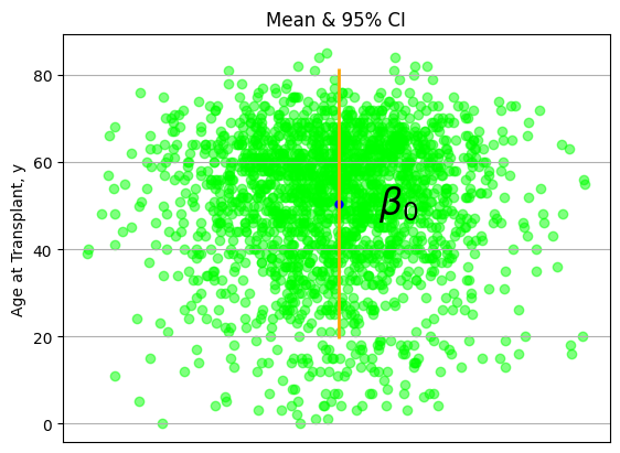
Which of these plots do you consider the most informative?
depends on your target audience
what are your goals (description vs. inference)?
both of the above
none of the above
06/30/2023#
591. success#
george lucas & will smith share a lot in common:
despite threats to a species at the intergalactic level
a superhero emerges to rescue an entire species
thus we have up-beat stories lines
this is essentially the difference between:
realism & idealism
\(\mu\) & \(\sigma\)
observed & expected
uses & abuses of history will seperate success from failure:
superhistorical & unhistorical
or a healthy balance thats just historical?
lets mesh these ideas over the next 12 months!
Show code cell source
import pandas as pd
import matplotlib.pyplot as plt
import numpy as np
import requests
import io

# Load the data from the URL using requests
url = 'https://raw.githubusercontent.com/jhustata/livre/main/transplants.txt'
response = requests.get(url)
content = response.content.decode('utf-8')
file = io.StringIO(content)
data = pd.read_csv(file, sep='\t')

# Extract relevant columns
age = data['age']
x = [1] * len(age)

# Calculate mean and standard deviation
mean_age = age.mean()
std_age = age.std()

# Calculate upper and lower bounds for 95% confidence interval
ub = mean_age + std_age * 1.96
lb = mean_age - std_age * 1.96

# Add jitter to x-axis values
x_jitter = x + np.random.normal(0, 0.02, size=len(x))

# Scatter plot of age with increased jitter
plt.scatter(x_jitter, age, c='lime', alpha=0.5)

# Mean point
plt.scatter(1, mean_age, c='blue', s=25)

# Confidence interval with thicker line
plt.errorbar(1, mean_age, yerr=[[mean_age - lb], [ub - mean_age]], color='orange', linewidth=2)

# Styling
plt.ylabel('Realism, %')
plt.title('Mean & 95% CI')
plt.text(1.01, mean_age, r'$\beta_0$', va='center', fontsize=24)
plt.xticks([])
plt.grid(True)

# Save the figure
plt.savefig('age_m_95ci.png')
plt.show()
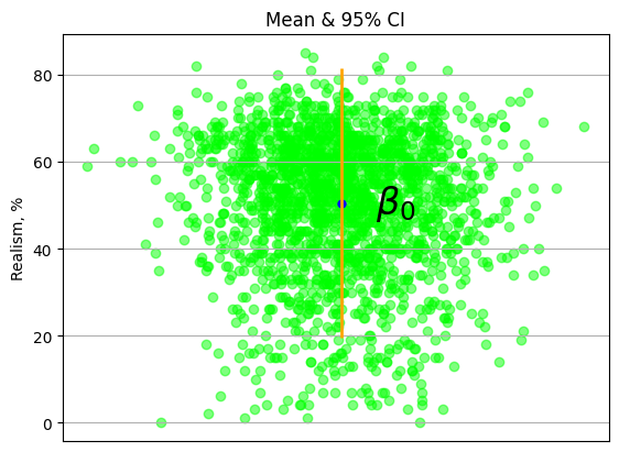
capture log close
log using age_o_age_e.log, replace
import delimited "https://raw.githubusercontent.com/jhustata/livre/main/transplants.txt", clear
regress rec_hgt_cm gender
label define gender_lab 0 "Male" 1 "Female"
label values gender gender_lab
lincom _cons
g male_m=r(estimate)
g male_lb= r(estimate) - e(rmse)*1.96
g male_ub= r(estimate) + e(rmse)*1.96
lincom _cons + gender
g female_m=r(estimate)
g female_lb= r(estimate) - e(rmse)*1.96
g female_ub= r(estimate) + e(rmse)*1.96
twoway  ///
   (scatter rec_hgt_cm gender if gender==0, ///
      yti("Height, cm", ///
	     orientation(horizontal) ///
	  ) ///
      text(210 0 "Male") ///
	  text(210 1 "Female") ///
      legend(off) ///
      mcolor(lime) ///
	  msymbol(oh) ///
	  jitter(30) ///
   ) ///
   (scatter rec_hgt_cm gender if gender==1, ///
     xscale(off) ///
     mcolor(lime) ///
	 msymbol(oh) ///
     jitter(30) ///
      xlab(-1(1)2 ///
	    -1 "" ///
	     0 "Male" ///
		 1 "Female" ///
		 2 "" ///
	  ) ///
   ) ///
   (scatter male_m gender if gender==0, ///
      msize(2) ///
	  mcolor(blue) ///
   )  ///
   (scatter female_m gender if gender==1, ///
      msize(2) ///
	  mcolor(blue) ///
   )  ///
   (rcap male_lb male_ub gender if gender==0, ///
      lcolor(orange_red) ///
   ) ///
   (rcap female_lb female_ub gender if gender==1, ///
      lcolor(orange_red) ///
   )
graph export twoway_hgt_gender.png, replace
log close
---------------------------------------------------------------------------------------------------------------------------------------------------------------------------
      name:  <unnamed>
       log:  /Users/d/Dropbox (Personal)/4d.∫δυσφορία.dt,ψ/4.describe/note/age_o_age_e.log
  log type:  text
 opened on:  30 Jun 2023, 00:40:31

. import delimited "https://raw.githubusercontent.com/jhustata/livre/main/transplants.txt", clear
(encoding automatically selected: ISO-8859-1)
(26 vars, 2,000 obs)

. regress rec_hgt_cm gender

      Source |       SS           df       MS      Number of obs   =     1,933
-------------+----------------------------------   F(1, 1931)      =    426.58
       Model |  70667.4243         1  70667.4243   Prob > F        =    0.0000
    Residual |  319890.062     1,931  165.660312   R-squared       =    0.1809
-------------+----------------------------------   Adj R-squared   =    0.1805
       Total |  390557.486     1,932  202.151908   Root MSE        =    12.871

------------------------------------------------------------------------------
  rec_hgt_cm | Coefficient  Std. err.      t    P>|t|     [95% conf. interval]
-------------+----------------------------------------------------------------
      gender |  -12.42026   .6013543   -20.65   0.000    -13.59963   -11.24089
       _cons |   173.4399   .3735802   464.26   0.000     172.7073    174.1726
------------------------------------------------------------------------------

. label define gender_lab 0 "Male" 1 "Female"

. label values gender gender_lab

. lincom _cons

 ( 1)  _cons = 0

------------------------------------------------------------------------------
  rec_hgt_cm | Coefficient  Std. err.      t    P>|t|     [95% conf. interval]
-------------+----------------------------------------------------------------
         (1) |   173.4399   .3735802   464.26   0.000     172.7073    174.1726
------------------------------------------------------------------------------

. g male_m=r(estimate)

. g male_lb= r(estimate) - e(rmse)*1.96

. g male_ub= r(estimate) + e(rmse)*1.96

. lincom _cons + gender

 ( 1)  gender + _cons = 0

------------------------------------------------------------------------------
  rec_hgt_cm | Coefficient  Std. err.      t    P>|t|     [95% conf. interval]
-------------+----------------------------------------------------------------
         (1) |   161.0197   .4712375   341.70   0.000     160.0955    161.9439
------------------------------------------------------------------------------

. g female_m=r(estimate)

. g female_lb= r(estimate) - e(rmse)*1.96

. g female_ub= r(estimate) + e(rmse)*1.96

. twoway  ///
>    (scatter rec_hgt_cm gender if gender==0, ///
>       yti("Height, cm", ///
>              orientation(horizontal) ///
>           ) ///
>       text(210 0 "Male") ///
>           text(210 1 "Female") ///
>       legend(off) ///
>       mcolor(lime) ///
>           msymbol(oh) ///
>           jitter(30) ///
>    ) ///
>    (scatter rec_hgt_cm gender if gender==1, ///
>      xscale(off) ///
>      mcolor(lime) ///
>          msymbol(oh) ///
>      jitter(30) ///
>       xlab(-1(1)2 ///
>             -1 "" ///
>              0 "Male" ///
>                  1 "Female" ///
>                  2 "" ///
>           ) ///
>    ) ///
>    (scatter male_m gender if gender==0, ///
>       msize(2) ///
>           mcolor(blue) ///
>    )  ///
>    (scatter female_m gender if gender==1, ///
>       msize(2) ///
>           mcolor(blue) ///
>    )  ///
>    (rcap male_lb male_ub gender if gender==0, ///
>       lcolor(orange_red) ///
>    ) ///
>    (rcap female_lb female_ub gender if gender==1, ///
>       lcolor(orange_red) ///
>    )

. graph export twoway_hgt_gender.png, replace
file /Users/d/Dropbox (Personal)/4d.∫δυσφορία.dt,ψ/4.describe/note/twoway_hgt_gender.png saved as PNG format

. log close
      name:  <unnamed>
       log:  /Users/d/Dropbox (Personal)/4d.∫δυσφορία.dt,ψ/4.describe/note/age_o_age_e.log
  log type:  text
 closed on:  30 Jun 2023, 00:40:33
---------------------------------------------------------------------------------------------------------------------------------------------------------------------------

592. stata-levels 🦀#
Show code cell source
import matplotlib.pyplot as plt
import numpy as np

# Create data for the skill and challenge levels
skill_levels = np.linspace(0, 10, 100)
challenge_levels = np.linspace(0, 10, 100)

# Define the flow channel boundaries
flow_channel = skill_levels

# Adjust the phase and amplitude of the sinusoid wave
phase = np.pi / 16  # Reducing the wavelength by a quarter
amplitude = 1.5
flow_channel += np.sin(skill_levels + phase) * amplitude

# Define the yellow zone boundaries
yellow_zone_low = flow_channel - 1.5
yellow_zone_high = flow_channel + 1.5

# Define the sinusoid function with the middle yellow line as its axis
sinusoid = flow_channel + np.sin(skill_levels + phase) * amplitude

# Define the anxiety and boredom areas
anxiety_area = np.where(challenge_levels > flow_channel, challenge_levels, np.nan)
boredom_area = np.where(challenge_levels < flow_channel, challenge_levels, np.nan)

# Plotting
plt.figure(figsize=(8, 6))

# Plot the anxiety and boredom areas
plt.fill_between(skill_levels, flow_channel, 10, color='red', alpha=0.3, label='Anxiety', interpolate=True)
plt.fill_between(skill_levels, 0, flow_channel, color='green', alpha=0.3, label='Boredom', interpolate=True)
plt.fill_between(skill_levels, yellow_zone_low, yellow_zone_high, color='yellow', alpha=0.3, label='Flow Channel', interpolate=True)

# Plot the sinusoid function
plt.plot(skill_levels, sinusoid, color='purple', linestyle='-')

# Add arrowhead to the sinusoid line (flipped direction)
plt.arrow(skill_levels[-2], sinusoid[-2], skill_levels[-1] - skill_levels[-2], sinusoid[-1] - sinusoid[-2],
          color='purple', length_includes_head=True, head_width=-0.15, head_length=-0.3)

# Plot the flow channel boundaries
plt.plot(skill_levels, flow_channel, color='yellow', linestyle='-')

# Set plot labels and title
plt.xlabel('Skill Level (Week)')
plt.ylabel('Challenge Level (Syllabus)')
plt.title('Stata Programming')

# Set plot limits and grid
plt.xlim(0, 10)
plt.ylim(0, 10)
plt.grid(True)

# Set tick labels
tick_labels = ['0', '2', '4', '6', '8', '10']
plt.xticks(np.linspace(0, 10, 6), tick_labels)
plt.yticks(np.linspace(0, 10, 6), tick_labels)

# Add text annotations to label the areas
plt.text(2.5, 7.5, 'Anxiety', color='black', ha='center', va='center', fontsize=12, bbox=dict(facecolor='pink', edgecolor='pink', boxstyle='round'))
plt.text(5, 5.1, 'Flow Channel', color='black', ha='center', va='center', fontsize=12, bbox=dict(facecolor='yellow', edgecolor='yellow', boxstyle='round'))
plt.text(7.5, 2.1, 'Boredom', color='black', ha='center', va='center', fontsize=12, bbox=dict(facecolor='lightgreen', edgecolor='lightgreen', boxstyle='round'))

# Display the plot
plt.show()
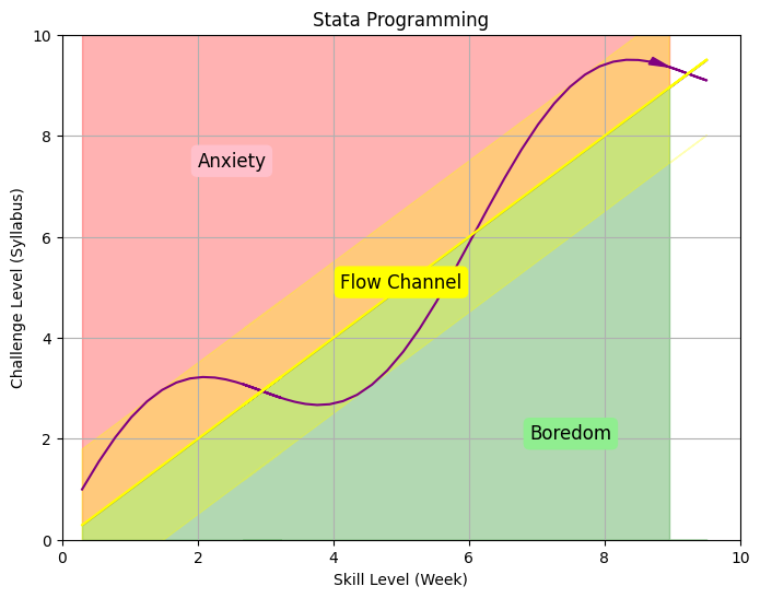
basic: right claw 🦀#
oneway scatter plot == observed, overlayed == expected
10ptimport data
1pthistogram or other command
1ptvarname syntax
1ptoptions
title
1ptytitle
1ptxtitle
1ptylab
1ptxlab
1pttext
1pt
documentation
1ptlogfile
graph export
twoway scatter plot == observed, overlayed == function(y = _cons + _b[x])
10ptimport data
1pttwoway, line, or other command
1ptvarlist syntax
1ptoptions
title
1ptytitle
1ptxtitle
1ptylab
1ptxlab
1pttext
1pt
documentation
1ptlogfile
graph export
visualize fit == observed, overlayed == _cons + _b1[x1] + _b2[x2] \(\cdots\) + _bN[xN]
10ptimport data
1pttwoway, line, or other command
1ptvarlist syntax
1ptoptions
title
1ptytitle
1ptxtitle
1ptylab
1ptxlab
1pttext
1pt
documentation
1ptlogfile
graph export
lincom over a twoway plot, segue’s into mixed models
basic documentation using a log-file
1pt
standard: left claw 🦀#
introduce program define, syntax varlist, exit, di in red, end, and catalog of errors
20ptcapture program drop name
1ptprogram define name
1ptsyntax varlist
1ptif conditional
1ptbracket option
1ptoptions
string/varlist
1ptnumeric/numlist
1pt
display in red
1ptcatalog error
1ptexit
1ptend
1ptuse command & display options
1ptworks on any dataset
1ptgives informative output when user gives incomplete input
1ptdefault output when user give bare-minimum syntax
1pt
generalize hardcoded scripts from basic-phase above to user-driven input
20ptditto
dofile script-insert
appropriate edits
loop over string & numeric values (e.g. over varlist *) and output .xlsxs (table1) & .png (figure1) output
20pt
multilingual: thorx & abd 🦀#
very rich documentation using jupyter- or quarto-books for stata, r, and python
3ptintroduce dyndoc, markdown, html, latex, and unix command-prompt
3ptdeploy .html to gh-pages, update book, establish workflow:
3ptlocally using jupyter labs, rstudio, and vscode
remotely using codespace, rstudio, etc
Show code cell source
import networkx as nx
import matplotlib.pyplot as plt
#import numpy as np
#import sklearn as skl
#

#plt.figure(figsize=[2, 2])
G = nx.DiGraph()
G.add_node("user",  pos = (550,500) )
G.add_node("system",  pos = (-550,500) )
G.add_node("program",  pos = (-2000, 960) )
G.add_node("syntax",  pos = (2000, 950) )
G.add_node("ado", pos = (-3000, 550) )
G.add_node("do", pos = (3000, 550) )
G.add_node("command", pos = (-1900, 150) )
G.add_node("queue", pos = (1900, 150) )
G.add_node("output", pos = (0,0))
G.add_node("dta", pos = (0, -475))
G.add_node("log", pos = (-1900, -475))
G.add_node("excel", pos = (-4000, -475))
G.add_node("word", pos = (1900, -475))
G.add_node("html", pos = (4000, -475))
G.add_node("publish", pos = (0, -950))
G.add_edges_from([ ("program","ado"), ("syntax", "do")])
G.add_edges_from([("ado", "command"), ("do", "queue") ])
G.add_edges_from([("command", "output"), ("queue", "output"),("output","excel"),("output","word"),("output","html")])
G.add_edges_from([("output","dta"),("output","log")])
G.add_edges_from([("dta","publish"),("log","publish"),("excel","publish"),("word","publish"),("html","publish")])
nx.draw(G,
        nx.get_node_attributes(G, 'pos'),
        with_labels=True,
        font_weight='bold',
        node_size = 4500,
        node_color = "lightblue",
        linewidths = 3)
ax= plt.gca()
ax.collections[0].set_edgecolor("#000000")
ax.set_xlim([-5000, 5000])
ax.set_ylim([-1000, 1000])
plt.show()
593. nietzsche#
uses & abuses of history
superhistorical, unhistorical, and mid-way historical
george lucas & will smith as exemplars extraordinaire of the balancing act
historical, which leads to highest levels of success
Show code cell source
import matplotlib.pyplot as plt
import numpy as np

# Create data for the skill and challenge levels
skill_levels = np.linspace(0, 10, 100)
challenge_levels = np.linspace(0, 10, 100)

# Define the flow channel boundaries
flow_channel = skill_levels

# Adjust the phase and amplitude of the sinusoid wave
phase = np.pi / 16  # Reducing the wavelength by a quarter
amplitude = 1.5
flow_channel += np.sin(skill_levels + phase) * amplitude

# Define the yellow zone boundaries
yellow_zone_low = flow_channel - 1.5
yellow_zone_high = flow_channel + 1.5

# Define the sinusoid function with the middle yellow line as its axis
sinusoid = flow_channel + np.sin(skill_levels + phase) * amplitude

# Define the anxiety and boredom areas
anxiety_area = np.where(challenge_levels > flow_channel, challenge_levels, np.nan)
boredom_area = np.where(challenge_levels < flow_channel, challenge_levels, np.nan)

# Plotting
plt.figure(figsize=(8, 6))

# Plot the anxiety and boredom areas
plt.fill_between(skill_levels, flow_channel, 10, color='red', alpha=0.3, label='Anxiety', interpolate=True)
plt.fill_between(skill_levels, 0, flow_channel, color='green', alpha=0.3, label='Boredom', interpolate=True)
plt.fill_between(skill_levels, yellow_zone_low, yellow_zone_high, color='yellow', alpha=0.3, label='Flow Channel', interpolate=True)

# Plot the sinusoid function
plt.plot(skill_levels, sinusoid, color='purple', linestyle='-')

# Add arrowhead to the sinusoid line (flipped direction)
plt.arrow(skill_levels[-2], sinusoid[-2], skill_levels[-1] - skill_levels[-2], sinusoid[-1] - sinusoid[-2],
          color='purple', length_includes_head=True, head_width=-0.15, head_length=-0.3)

# Plot the flow channel boundaries
plt.plot(skill_levels, flow_channel, color='yellow', linestyle='-')

# Set plot labels and title
plt.xlabel('Film Portrayal (Wish)')
plt.ylabel('Challenge Level (Life)')
plt.title('Audience Feelings (Ratings)')

# Set plot limits and grid
plt.xlim(0, 10)
plt.ylim(0, 10)
plt.grid(True)

# Set tick labels
tick_labels = ['0', '2', '4', '6', '8', '10']
plt.xticks(np.linspace(0, 10, 6), tick_labels)
plt.yticks(np.linspace(0, 10, 6), tick_labels)

# Add text annotations to label the areas
plt.text(2.8, 7.9, 'Anxiety (Realism) Critical, xline', color='black', ha='center', va='center', fontsize=12, bbox=dict(facecolor='pink', edgecolor='pink', boxstyle='round'))
plt.text(5, 5.1, 'Flow (Pragmaticism) Monumental, x=y', color='black', ha='center', va='center', fontsize=12, bbox=dict(facecolor='yellow', edgecolor='yellow', boxstyle='round'))
plt.text(6.2, 2.1, 'Boredom (Idealism) Antiquarian, yline', color='black', ha='center', va='center', fontsize=12, bbox=dict(facecolor='lightgreen', edgecolor='lightgreen', boxstyle='round'))

# Display the plot
plt.show()
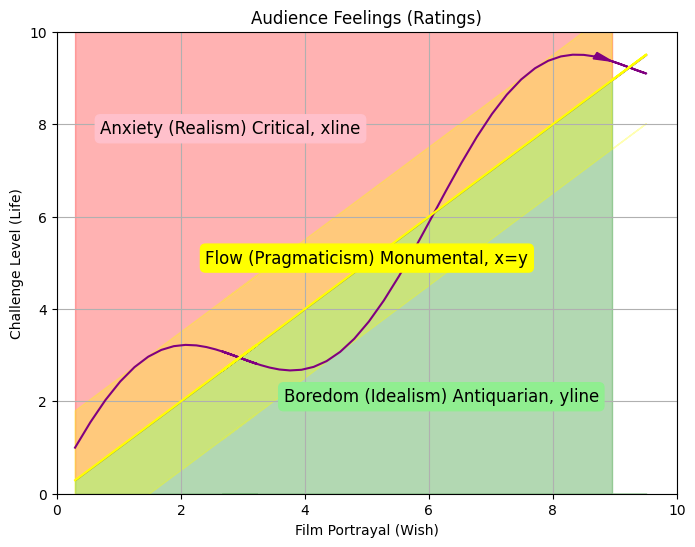
George Lucas in his debut and sophomore films moves the audience from
anxietytoflowBel-Air reboot of Will Smith’s The Fresh Prince moves the audience from
flowtoanxietyThe direction of boxoffice and streaming outcomes are mostly predicatable in both cases
594. prudence?#
realism
idealism
pragmaticism
596. cluster#
# andrew
ssh amuzaal1@jhpce01.jhsph.edu
moZart1234

# seasons
read_dta("/dcs04/legacy-dcs01-igm/segevlab/data/srtr/srtr2211/saf/stata/donor_live.dta")

# risk of esrd
~amassie/mock_cdrg/

# data: File paths go here
# Global path

global.path <- "../srtr2106/Stata/" #global.path <- "~amassie/mock_cdrg/"

# donor_live data goes on the following line
d1 <- read_dta(paste0(global.path,"donor_live.dta")) %>%
       select(all_of(vars.donor_live.dta), all_of(vars.don_liv_cms.dta))
597. shadrack#
usurp/inspiration/flex
worship/abuse/critique
satiate/commune/epicurus
598. verb#
do
be
enjoy
599. dude-vs-ennui#
“Looking for work in order to be paid: in civilized countries today almost all men are at one in doing that. For all of them work is a means and not an end in itself. Hence they are not very refined in their choice of work, if only it pays well. But there are, if only rarely, men who would rather perish than work without any pleasure in their work. They are choosy, hard to satisfy, and do not care for ample rewards, if the work itself is not to be the reward of rewards. Artists and contemplative men of all kinds belong to this rare breed, but so do even those men of leisure who spend their lives hunting, traveling, or in love affairs and adventures. All of these desire work and misery only if it is associated with pleasure, and the hardest, most difficult work if necessary. Otherwise their idleness is resolute, even if it spells impoverishment, dishonor, and danger to life and limb. They do not fear boredom as much as work without pleasure.” –Gaya Scienza
600. vioplot#
From: Yyy <yyye@jhmi.edu>
Date: Friday, June 30, 2023 at 4:35 PM
To: Xxx <xxx@jh.edu>
Subject: Re: HTML format =)
I’ m delighted by this news! Enjoy your weekend, Xxx! 😊

From: Xxx <malzahr1@jh.edu>
Date: Friday, June 30, 2023 at 4:34 PM
To: Yyy <yyy@jhmi.edu>
Subject: RE: HTML format =)
Excellent!! I have been trying since the morning, and I just used the first line you sent to me in STATA (ssc install vioplot), and it worked !!! This is great!
Without your help, I would spend the weekend trying, so I can enjoy it now =)

Thank you so much.

Best,
Xxx


From: Yyy <yyy@jhmi.edu>
Date: Friday, June 30, 2023 at 4:12 PM
To: Xxx <xxx@jh.edu>
Subject: Re: HTML format =)
Here’s a do-file demonstrating how to use the command.

But please review the classnotes:

   https://jhustata.github.io/livre/chapter1.html#overview

This is a third-party .ado file that you MUST ask other uses to first install.

From: Xxx <xxx@jh.edu>
Date: Friday, June 30, 2023 at 4:00 PM
To: Yyy <yyy@jhmi.edu>
Subject: RE: HTML format =)
May I be wrong..

It's to create a Violin plot the same as I attached.

Here is my code;
foreach v in mean_SS RR_total score {

              gen `v'_R = `v' if type == 1
              gen `v'_S = `v' if type == 5
              local title: var label `v'
              vioplot `v'_R `v'_S, over(Place) title("`title'") graphregion(color(white)) name(vio_`v', replace)
              graph export ".../vio_`v'.png", replace
}

Thanks,


From: Yyy <yyy@jhmi.edu>
Sent: Friday, June 30, 2023 12:24 PM
To: Xxx <xxx@jh.edu>
Subject: Re: HTML format =)

I’ve never heard of vioplot

From: Xxx <xxx@jh.edu>
Date: Friday, June 30, 2023 at 12:23 PM
To: Yyy <yyy@jhmi.edu>
Subject: RE: HTML format =)
Hi again,

I hope you are doing well. I am sorry for bothering you, but today I will submit all my STATA work, so this may be the last question =)

I want to create a plot using Vioplot, but I am encountering an issue in that the command Vioplot is unrecognized. In this case, what should I do?

I tried to use this code to install
ssc install violinplot, replace
and also these

. ssc install dstat, replace
. ssc install moremata, replace
. ssc install palettes, replace
. ssc install colrspace, replace


Unfortunately, it did not work. Knowing that my STATA version is 17.

Thank you in advance for your time. I really appreciate it.

Best,
Xxx


From: Yyy <yyy@jhmi.edu>
Sent: Monday, June 26, 2023 1:22 PM
To: Xxx <xxx@jh.edu>
Subject: Re: HTML format =)

I’m delighted to know that you are experimenting with this. Do you mind sharing two things with me so that I understand what you are dealing with:
1.	The entire dyndoc command you are typing into the Stata window
2.	The file you are converting into .html
This will allow me to quickly figure out if there is a syntax issue or perhaps a “markup” issue (e.g. remove <<dd_graph>> if there is no graphical output)

From: Xxx <xxx@jh.edu>
Date: Monday, June 26, 2023 at 1:13 PM
To: Yyy <yyy@jhmi.edu>
Subject: HTML format =)
Hi Yyy,

I hope you are doing well. Taking the STATA course with you was beneficial, and I will definitely join your course next year.

Regarding converting the do file in STATA to HTML, I have been trying this since morning using my own code, not transplants data, and I am facing this issue (dd_graph tag failed to export graph) because my code did not include any exploring graph only some calculations. I would greatly appreciate it if you could help me to solve it; I really would convert my code to html file. It's so impressive =)

Thank you in advance for your time.

Xxx
sysuse auto, clear
ssc install vioplot
foreach v in mpg headroom turn {
    gen `v'_R = `v' if foreign == 0
    gen `v'_S = `v' if foreign == 1
    local title: variable label `v'
    vioplot `v'_R `v'_S, over(rep78) title("`title'") graphregion(color(white)) name(vio_`v', replace)
    graph export "vio_`v'.png", replace
}
which vioplot
. sysuse auto, clear
(1978 automobile data)

. ssc install vioplot
checking vioplot consistency and verifying not already installed...
all files already exist and are up to date.

. foreach v in mpg headroom turn {
2.     gen `v'_R = `v' if foreign == 0
3.     gen `v'_S = `v' if foreign == 1
4.     local title: variable label `v'
5.     vioplot `v'_R `v'_S, over(rep78) title("`title'") graphregion(color(white)) name(vio_`v', replace)
6.     graph export "vio_`v'.png", replace
7. }
(22 missing values generated)
(52 missing values generated)
file /Users/d/Dropbox (Personal)/4d.∫δυσφορία.dt,ψ/4.describe/note/vio_mpg.png saved as PNG format
(22 missing values generated)
(52 missing values generated)
file /Users/d/Dropbox (Personal)/4d.∫δυσφορία.dt,ψ/4.describe/note/vio_headroom.png saved as PNG format
(22 missing values generated)
(52 missing values generated)
file /Users/d/Dropbox (Personal)/4d.∫δυσφορία.dt,ψ/4.describe/note/vio_turn.png saved as PNG format

. which vioplot
/Users/d/Library/Application Support/Stata/ado/plus/v/vioplot.ado
*! version 1.1.5  24may2012 by austinnichols@gmail.com and nwinter@virginia.edu
*! create violin plots

.
end of do-file

.


601. conscience#
To stand in the midst of … this whole marvelous uncertainty and rich ambiguity in existence without questioning, without trembling with the craving and the rapture of such questioning … that is what I feel to be contemptible, and this is the feeling for which I look first in everybody. Some folly keeps persuading me that every human has this feeling just because he is human
602. voyage#
“A human being who strives for something great considers everyone he meets on his way either as a means or as a delay and obstacle — or as a temporary resting place.”
means
obstacle
delay
603. happiness#
What is good? —Everything that enhances people’s feelings of power, will to power, power itself.
What is bad? —Everything stemming from weakness.
What is happiness? —The feeling that power is growing, that some resistance has been overcome.
Not contentedness, but more power;
Not peace, but war;
Not virtue, but prowess…
604. prophylaxis#
We have art in order not to die of the truth
605. eccehomo#
know my fate. One day my name will be associated with the memory of something tremendous — a crisis without equal on earth, the most profound collision of conscience, a decision that was conjured up against everything that had been believed, demanded, hallowed so far. I am no man, I am dynamite.
606. nietzsche#
Show code cell source
import requests
from bs4 import BeautifulSoup

# URLs to scrape
urls = [
    "https://www.gutenberg.org/files/52190/52190-h/52190-h.htm",
    "https://muzaale.github.io/book/bilowozo.html#id173"
]

# Terms to search for (English and German variations)
search_terms = ["caesar", "cesare", "borgia", "napoleon"]

# Function to check if a given text contains any of the search terms
def check_for_terms(text):
    for term in search_terms:
        if term.lower() in text.lower():
            return True
    return False

# Scrape the URLs and search for the terms
for url in urls:
    response = requests.get(url)
    soup = BeautifulSoup(response.content, "html.parser")
    paragraphs = soup.find_all("p")

    print(f"Searching {url}...\n")
    found_count = 0

    for paragraph in paragraphs:
        if check_for_terms(paragraph.get_text()):
            print(paragraph.get_text())
            found_count += 1

    print(f"\n{found_count} references found in {url}\n{'-' * 50}\n")